Using the calculus we have developed, it is usually straightforward to write the equations that critical points must satisfy. Activity 5.2.1 also shows the problem: those equations may be nonlinear and difficult or impossible to solve exactly. This is different from the linear systems in Unit 2, where Gaussian elimination gave a systematic exact method.
The positive scalar \(\alpha\) is the step size. The minus sign moves in a direction where \(f\) initially decreases. The method does not automatically converge; the function, starting point, and step size matter.
Let \(f\) be a scalar-valued function. Then if \(\mathbf{v}\) is a unit vector, the directional derivative of \(f\) in the direction of the vector \(\mathbf{v}\text{,}\) denoted \(D_{\mathbf{v}} f\text{,}\) is defined as
The directional derivative represents the rate of change of the function \(f\) at the point \(\mathbf{a}\) in the direction of the unit vector \(\mathbf{v}\text{.}\) For a function \(f(x,y)\) of two variables, the directional derivative \(D_{\mathbf{v}} f(\mathbf{a})\) is the slope of the tangent line to the curve obtained by intersecting the surface \(z = f(x,y)\) with the plane containing both the line passing through \(\mathbf{a}\) with direction vector \(\mathbf{v}\text{,}\) and the \(z\) axis.
Despite partial derivatives being a special case of directional derivatives, in most circumstances we can compute directional derivatives using partial derivatives, or equivalently, the gradient.
Suppose \(f\) is a function differentiable at a point \(\mathbf{a}\text{.}\) Then for each unit vector \(\mathbf{v}\text{,}\)\(D_{\mathbf{v}} f(\mathbf{a}) = \nabla f(\mathbf{a}) \cdot \mathbf{v}\text{.}\)
We apply the chain rule. We note that \(D_{\mathbf{v}} f(\mathbf{a})\) is equal to the derivative of the function \(g(t) = f(\mathbf{a} + t \mathbf{v})\) at \(t = 0\) (both derivatives are defined as the same limits). If we write \(\mathbf{c}(t) = \mathbf{a} + t \mathbf{v}\text{,}\) then \(g = f \circ \mathbf{c}\text{.}\) But the chain rule (Theorem 3.6.4) implies that
The largest listed directional derivative occurs in direction \(\mathbf{v}_3\text{,}\) the direction of the gradient. The smallest occurs in direction \(\mathbf{v}_4\text{,}\) the direction opposite the gradient. This is the Unit 1 dot product measuring alignment: larger positive alignment gives larger directional derivative.
Find the directional derivative of \(f\) at the point \((-1,3)\) in the direction of the vector \((-1,\sqrt{3})\text{.}\) That is, compute \(D_{\mathbf{v}} f(-1,3)\text{,}\) where \(\mathbf{v}\) is the unit vector in the direction of \((-1,\sqrt{3})\text{.}\)
Use the gradient of the function \(f(x,y) = x^3y\) to find the directional derivative of \(f\) at \((2,1)\) in the direction of the unit vector which we placed at \((2,1)\) points in the direction of the point \((3,5)\text{.}\)
The unit vector pointing in the direction from \((2,1)\) to \((3,5)\) is the unit vector pointing in the same direction as the vector \((3-2,5-1) = (1,4)\text{.}\) This vector has magnitude \(\sqrt{1^2 + 4^2} = \sqrt{17}\text{,}\) so the unit vector pointing in this direction is equal to
We have already verified the theorem when \(\nabla f(\mathbf{a}) = \mathbf{0}\) in Theorem 5.2.3. When \(\nabla f(\mathbf{a}) \neq \mathbf{0}\text{,}\)Theorem 5.2.3 and the Cauchy-Schwarz Inequality Theorem 4.1.2 says that
where the inequality is an equality precisely when \(\mathbf{u}\) either points in the direction of \(\nabla f(\mathbf{a})\text{,}\) or points in the opposite of this direction. But when \(\mathbf{u}\) points in the direction of \(\nabla f(\mathbf{a})\text{,}\) i.e., when \(\mathbf{u} = \nabla f(\mathbf{a}) / \| \nabla f(\mathbf{a}) \|\text{,}\) we have
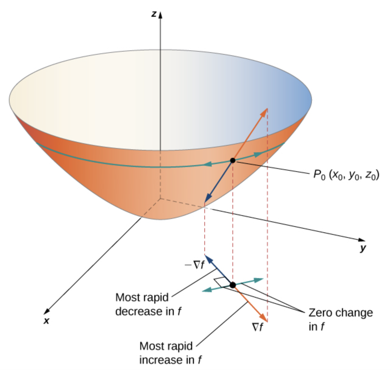
A bowl-shaped surface is shown above the \(xy\)-plane with a point \(P_0(x_0,y_0,z_0)\) on the side of the surface. On the plane below, arrows based at the corresponding point show \(\nabla f\) for most rapid increase, \(-\nabla f\) for most rapid decrease, and perpendicular directions for zero change in \(f\text{.}\) Dashed vertical guide lines connect the point on the surface to its location in the domain.
Find the direction for which the directional derivative of \(f(x,y) = 3x^2 - 4xy + 2y^2\) at \((-2,3)\) is a maximum. What is the maximum value of the directional derivative?
Theorem 5.2.4 tells us that the directional derivative \(D_{\mathbf{v}} f\) is maximized when \(\mathbf{v}\) is the unit vector pointing in the direction of \((-24,20)\text{.}\) Since \((-24,20)\) has magnitude \(\sqrt{(-24)^2 + (20)^2} = \sqrt{976}\text{,}\) we see the direction which maximizes the directional derivative is
We now return to the gradient descent algorithm, a method for trying to approximate the local minima of a function \(f\text{.}\) The algorithm works as follows:
Start at an initial point \(\mathbf{x}_0\text{.}\)
Move in the direction of the negative gradient: set \(\mathbf{x}_1 = \mathbf{x}_0 - \alpha_0 \nabla f(\mathbf{x}_0)\text{,}\) where \(\alpha_0 > 0\) is a step size (or learning rate) parameter.
Repeat steps 2-3 with step sizes \(\alpha_1, \alpha_2, \dots\) to successively define points \(\mathbf{x}_2 = \mathbf{x}_1 - \alpha_1 \nabla f(\mathbf{x}_1)\text{,}\)\(\mathbf{x}_3 = \mathbf{x}_2 - \alpha_2 \nabla f(\mathbf{x}_2)\text{,}\) and so on, with the hope that these points converge to a local minimum.
Intuitively, gradient descent works because each successive value \(\mathbf{x}_k\) is obtained by shifting the previous value \(\mathbf{x}_{k-1}\) in the direction in which the function \(f\) decreases the fastest. The algorithm is likely to find local minima of a function \(f\text{,}\) although a rigorous analysis of this algorithm is quite involved.
The learning rate is alpha. The vector grad_f(x) must have the same shape as x, because the update subtracts one vector from another. If the minus sign were a plus sign, the update would move in the direction of steepest increase rather than steepest decrease.
using gradient descent. Use the starting point \(\mathbf{x}_0 = (0,0)\text{,}\) a constant step size of \(0.1\text{,}\) and stop after computing \(\mathbf{x}_3\text{.}\) You may use a calculator to perform these computations.
We note that for this function, we can precisely compute that \(f\) has a critical point at \((-9, -16/3)\text{,}\) which by the second derivative test is a local minimum. So \(\mathbf{x}_3\) is not a good approximation to the local minimum. But if we continued to iterate this algorithm, we would find that the points \(\mathbf{x}_k\) for, say, \(k \geq 1000\text{,}\) are very close to the true minimum of the function.
This algorithm can be rather cumbersome to compute by hand, but if the gradient of a function is easily determined, can be easily done to a large number of iterations on a computer.
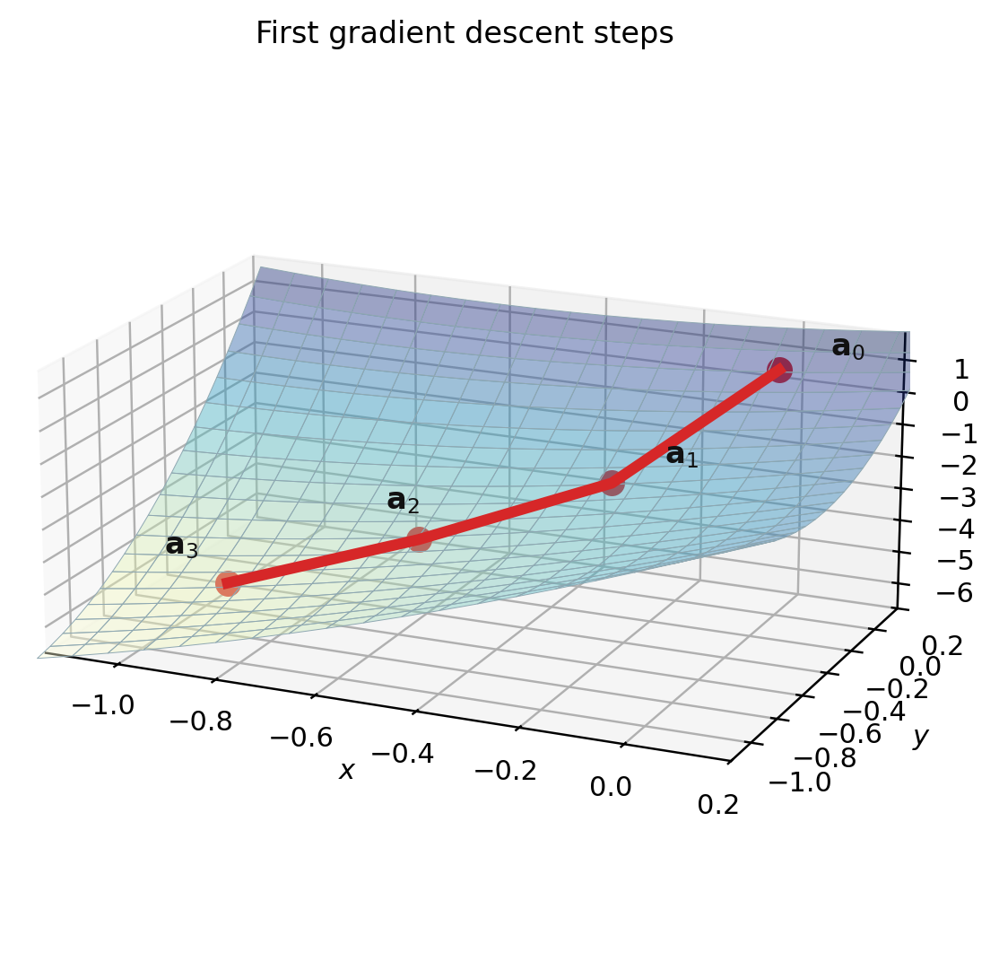
The figure shows a side view of the surface \(z=f(x,y)\) for \(f(x,y)=x^2-3xy+3y^2+5y+2x\) over a small region near the origin. Four red points labeled \(\mathbf{a}_0\text{,}\)\(\mathbf{a}_1\text{,}\)\(\mathbf{a}_2\text{,}\) and \(\mathbf{a}_3\) are connected by red line segments on the surface, showing the first three gradient descent steps from \((0,0)\text{.}\)
Figure5.2.8.Initial steps of gradient descent for \(f(x,y)=x^2-3xy+3y^2+5y+2x\) with starting point \(\mathbf{a}_0 = (0, 0)\text{.}\) The point \(\mathbf{a}_n\) is determined by the rule \(\mathbf{a}_n = \mathbf{a}_{n-1} - (0.1) \nabla f(\mathbf{a}_{n-1})\text{.}\) Adapted from: Stanford’s MATH 51 textbook.