We compute the partial derivative in \(x\) of an expression precisely by treating the \(y\)-variable as a constant, and differentiating in \(x\text{.}\) Similarly, we compute the partial derivative in \(y\) by treating the \(x\)-variable as a constant.
Given a function \(f(x,y)\) and \(b \in \R\text{,}\) the slice of the function \(f\) in the plane \(y = b\) is the function \(g: \R \to \R\) given by \(g(x) = f(x,b)\text{.}\) Similarly, for \(x \in \R\) the slice of \(f\) in the plane \(x = a\) is the function \(g: \R \to \R\) given by \(g(y) = f(a,y)\text{.}\)
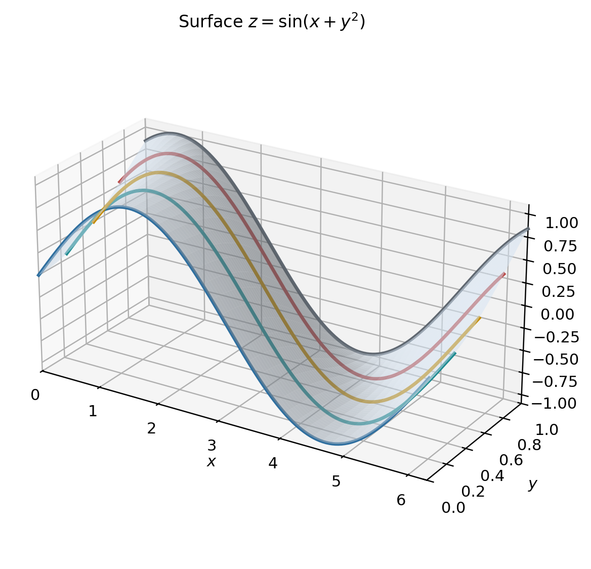
Geometrically, the slice of a function \(f\) in the plane \(y = b\) corresponding to intersecting the surface given by the equation \(z = f(x,y)\) with the plane \(y = b\text{,}\) creating a curve in this plane.
The figure shows a translucent blue surface for \(z = \sin(x+y^2)\) over \(0 \leq y \leq 1\text{.}\) Five colored curves lie on the surface at fixed values \(y=0\text{,}\)\(y=0.25\text{,}\)\(y=0.5\text{,}\)\(y=0.75\text{,}\) and \(y=1\text{,}\) illustrating how the slice \(z=\sin(x+b^2)\) shifts as \(b\) changes.
Figure3.3.7.The graph of \(f(x,y) = \sin(x + y^2)\) showing slices at different values of \(y\text{.}\) Each curve represents the function \(f(x,y)\) for a fixed value of \(y\text{.}\) Adapted from: Stanford’s MATH 51 textbook
This is the slope of the curve in the \(xz\) plane obtained by intersecting the surface \(z = 16 - x^2 - y^2\) with the plane defined by the equation \(y = 2\text{,}\) at the point \((1,2,11)\text{.}\) That is, the tangent line of the curve at this point is given by \(z - 11 = -2 ( x - 1 )\text{.}\)
This is the slope of the curve in the \(yz\) plane obtained by intersecting the surface \(z = 16 - x^2 - y^2\) with the plane defined by the equation \(x = 1\text{,}\) at the point \((1,2,11)\text{.}\) That is, the tangent line of the curve at this point is given by \(z - 11 = -4 ( y - 2 )\text{.}\)
Activity3.3.10.Reading partial derivatives along a horizontal line (U3-LO3).
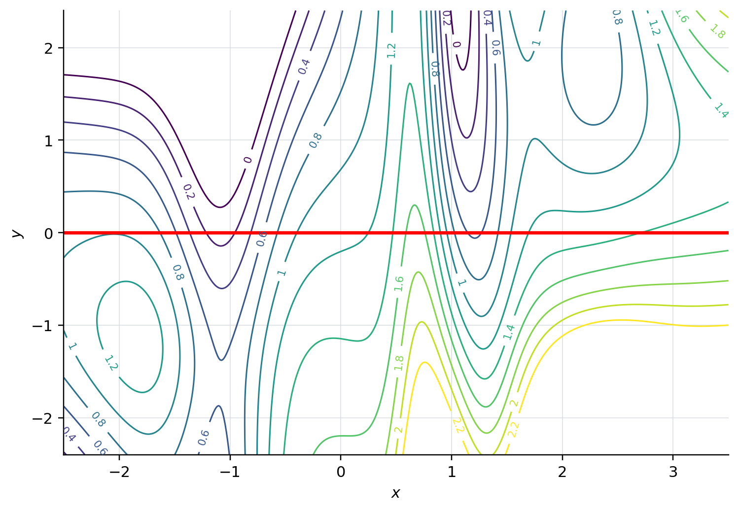
Consider the contour plot shown in Figure 3.3.11 for a function \(F\) with contour lines at increments of \(0.2\text{.}\) In particular, consider the curve obtained from the slice \(y = 0\text{,}\) indicated by the red line in Figure 3.3.11. By interpreting the contour plot, what can we say about the slopes of this curve, or equivalently, the values of \(F_x\) on this line?
The contour plot shows a synthetic function with labeled level curves spaced by \(0.2\text{.}\) A thick red horizontal line marks \(y=0\text{,}\) so the intersections of that line with the contour curves can be compared with the one-variable slice along \(y=0\text{.}\)
Figure3.3.11.A contour plot for a function with increments of \(0.2\text{.}\) The line \(y = 0\) is indicated in red. Adapted from: Stanford’s MATH 51 textbook
Here is some of the information we can read from the contour plot:
Between \(x = -1\) and \(x = 0\text{,}\) the contour values increase (from about \(0.2\) to \(1\)), indicating \(F_x > 0\) in this region (the function \(F\) is increasing).
Near \(x = 1\text{,}\) the contour lines are very close together, and the contour values decrease, indicating the \(F_x \lt 0\text{,}\) and that the magnitude of \(F_x\) is large (the curve slopes steeply downward).
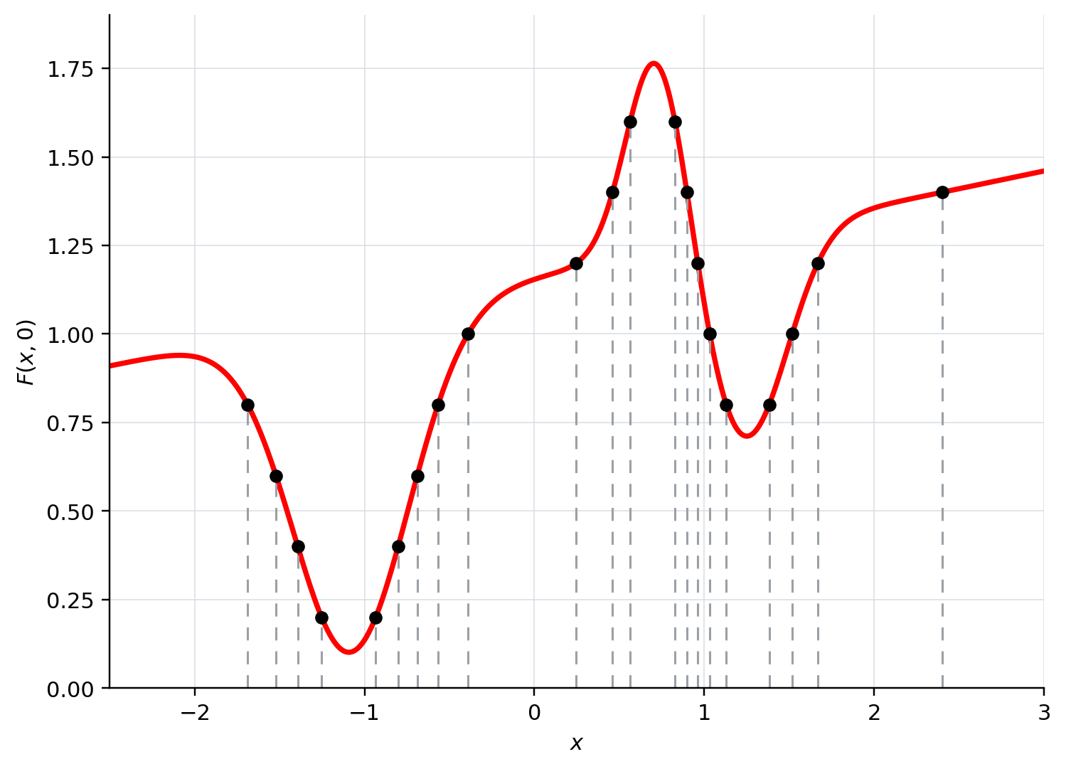
The graph shows the slice \(F(x,0)\) as a red curve. Black points mark where the slice reaches contour levels in increments of \(0.2\text{,}\) and gray dashed vertical lines run from the \(x\)-axis up to those points.
Figure3.3.12.The slice of the function \(F(x,y)\) where \(y = 0\text{.}\) The dashed lines correspond to increments of \(0.2\) in the \(x\)-axis. Adapted from: Stanford’s MATH 51 textbook
Activity3.3.13.Reading partial derivatives along a vertical line (U3-LO3).
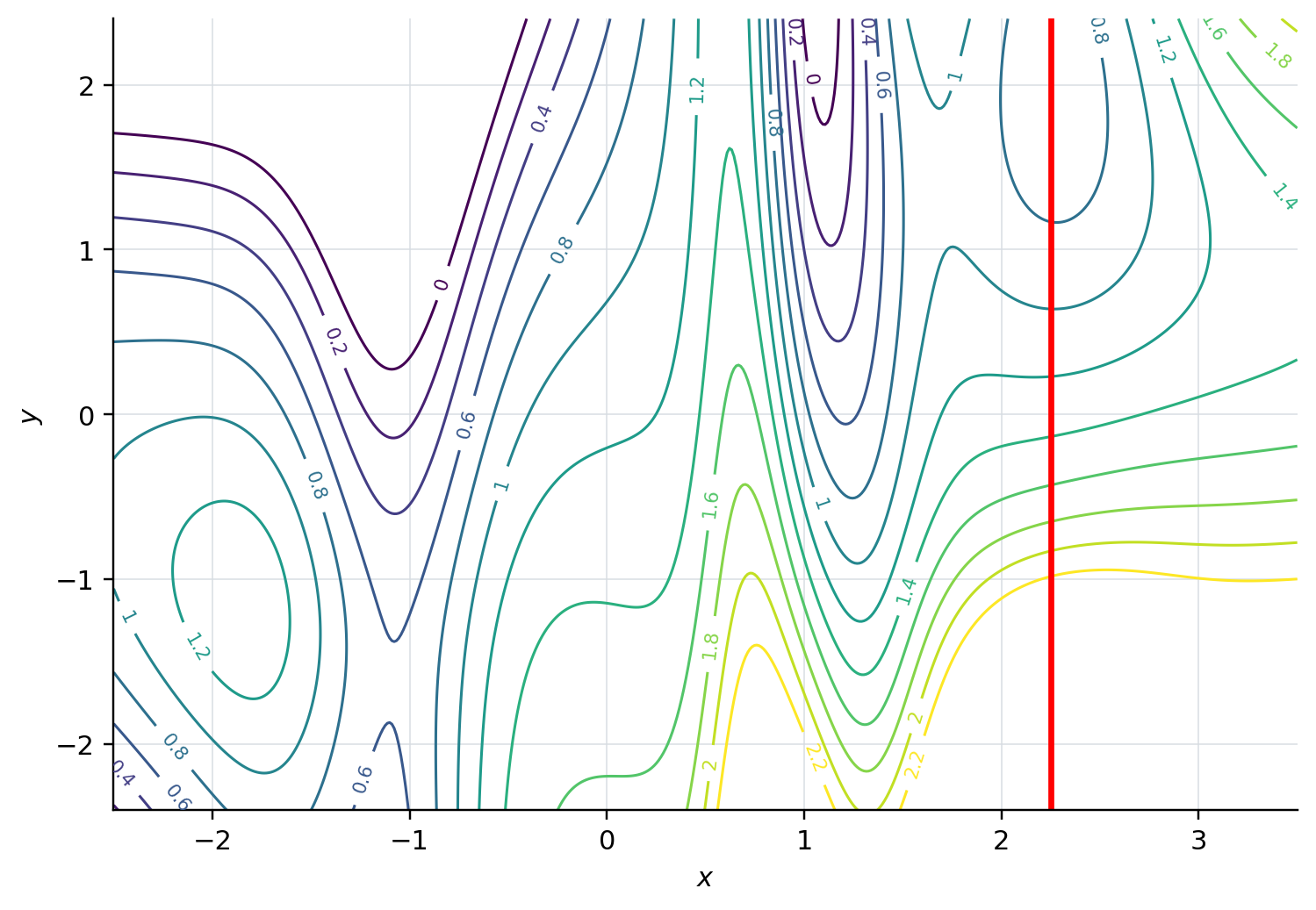
Consider Figure 3.3.14, which is the same contour plot as in Figure 3.3.11, but with the vertical line \(x = 2.25\) indicated instead. As in Activity 3.3.10, read off the behaviour of the partial derivatives \(F_y\) from the contour plot.
The contour plot shows the same synthetic function as the preceding contour figure, with labeled level curves spaced by \(0.2\text{.}\) A thick red vertical line marks \(x=2.25\text{,}\) so changes in contour values along this vertical slice can be read from bottom to top.
Figure3.3.14.A contour plot with increments of \(0.2\text{,}\) with the vertical line \(x = 2.25\) highlighted in red. Adapted from: Stanford’s MATH 51 textbook
Generally, the spacing of contour lines corresponds to the magnitude of partial derivatives, and the sign of the partial derivatives corresponds to whether the function increases or decreasing in that direction.
Activity3.3.15.Checking derivative signs against a contour plot (U3-LO3).
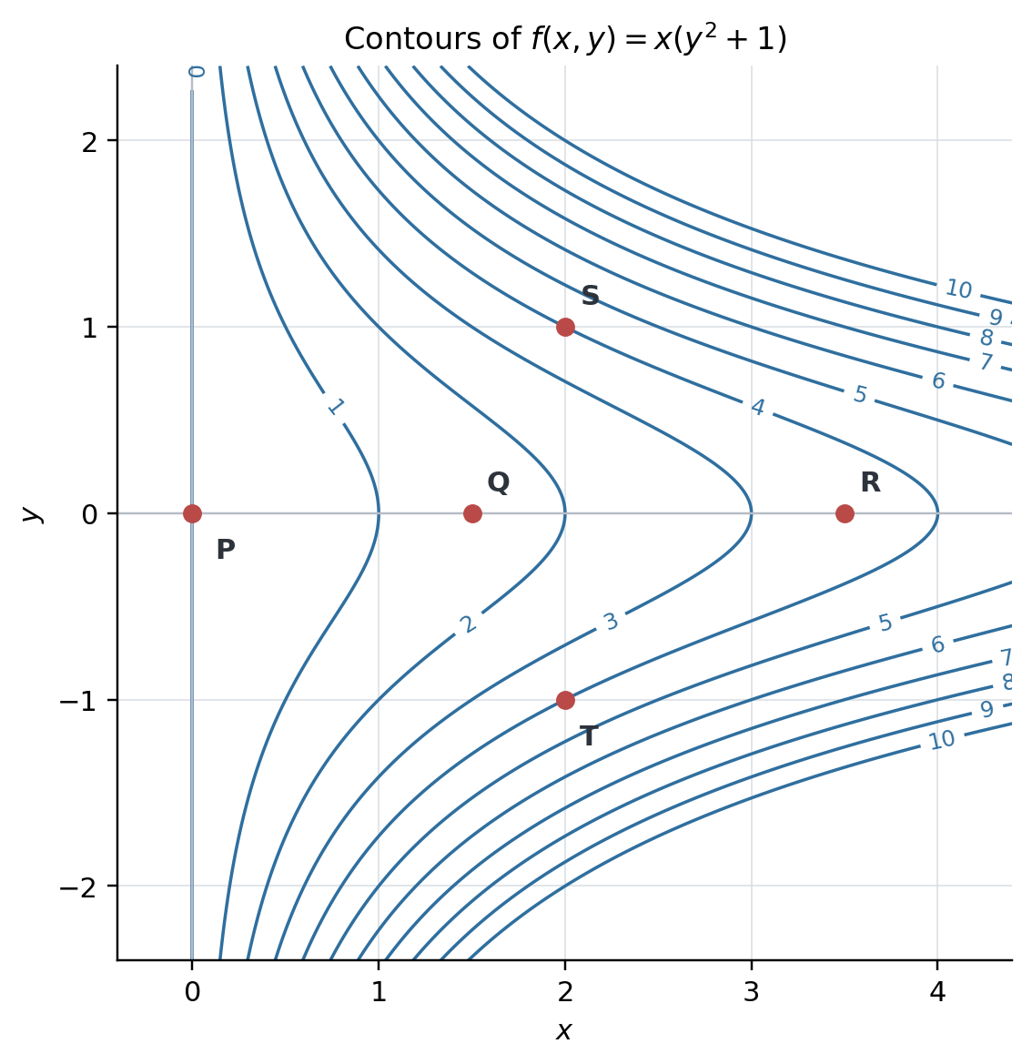
Consider the function \(f(x,y) = x(y^2 + 1)\text{,}\) whose contour plot is indicated in Figure 3.3.16. Five points are marked on the plot: \(P = (0,0)\text{,}\)\(Q = (3/2,0)\text{,}\)\(R = (7/2,0)\text{,}\)\(S = (2,1)\text{,}\) and \(T = (2,-1)\text{.}\) For each of these five points, determine from the contour plot whether \(f_x\) is positive, negative, or zero, and whether \(f_y\) is positive, negative, or zero. Then calculate these derivatives exactly and check whether your observations were correct.
The contour plot shows level curves of \(f(x,y)=x(y^2+1)\) for levels from \(0\) through \(10\) in steps of \(1\text{.}\) The level curves are symmetric across the \(x\)-axis and bend to the right as \(|y|\) increases. The marked points are \(P=(0,0)\text{,}\)\(Q=(3/2,0)\text{,}\)\(R=(7/2,0)\text{,}\)\(S=(2,1)\text{,}\) and \(T=(2,-1)\text{.}\)
Figure3.3.16.Contour plot for \(f(x,y) = x(y^2 + 1)\) with increments of \(1\text{,}\) and five points \(P\text{,}\)\(Q\text{,}\)\(R\text{,}\)\(S\text{,}\) and \(T\) indicated. Adapted from: Stanford’s MATH 51 textbook
At all five points, \(f_x > 0\) because the contour values increase as increase values of \(x\text{.}\) The contour lines around points \(S\) and \(T\) are more tightly packed than around \(P\text{,}\)\(Q\text{,}\) and \(R\text{,}\) indicating that \(f_x\) has larger magnitude at \(S\) and \(T\) than at \(P\text{,}\)\(Q\text{,}\) and \(R\text{.}\)
At the point \(P\text{,}\)\(f_y = 0\) since the contour line passing through \(P\) is a straight vertical line. It is not possible to determine the sign of \(f_y\) at the points \(Q\) and \(R\text{,}\) but we know the value of \(f_y\) must be small since the contour lines are more spread out than anywhere else in the plot. At the point \(S\text{,}\)\(f_y > 0\text{,}\) since the contour values increase as we increase in \(y\) values. At the point \(T\text{,}\)\(f_y \lt 0\) since the contour values decrease.
If the variables \(x_1,\dots,x_n\) are denoted using different symbols, these symbols might also be used to denote the partial derivatives instead. For instance, in \(\R^3\text{,}\) we might write a function as \(f(x,y,z)\text{,}\) and then the three partial derivatives of \(f\) may be denoted using any of the following four notations:
\(\frac{\partial f}{\partial x}\text{,}\)\(\frac{\partial f}{\partial y}\text{,}\) and \(\frac{\partial f}{\partial z}\text{.}\)
As for functions of two variables, we can calculate these derivatives by treating all variables but that we are taking the partial derivative of as constants.
Given a scalar-valued function \(f\text{,}\) the partial derivatives of \(f\) (where defined) are also scalar-valued functions, so we can consider partial derivatives of that function as well, which leads to higher order partial derivatives.
If \(f\) is a function of two variables, then the second-order partial derivatives of \(f\) are defined as:
The derivative \(f_{xx}\) or \(\frac{\partial^2 f}{\partial x^2}\text{,}\) obtained by taking the partial derivative of \(f\) twice in the \(x\) variable.
The derivative \(f_{yx}\) or \(\frac{\partial^2 f}{\partial y \partial x}\text{,}\) obtained by first differentiating \(f\) in the \(x\) variable, and then differentiating \(f\) in the \(y\) variable.
The derivative \(f_{xy}\text{,}\) or \(\frac{\partial^2 f}{\partial x \partial y}\text{,}\) obtained by first differentiating \(f\) in the \(y\) variable, and then differentiating \(f\) in the \(x\) variable.
Similarly, for a function \(f(x_1,\dots,x_n)\text{,}\) the higher derivatives of \(f\) are defined as \(f_{x_i x_j} = \frac{\partial^2 f}{\partial x_i \partial x_j}\) for \(1 \leq i,j \leq n\text{,}\) obtained by first differentiating \(f\) in the variable \(x_j\text{,}\) and then differentiating \(f\) in the \(x_i\) variable.
Suppose a scalar-valued function \(f\) is defined in an open ball \(B\) that contains a point \(\mathbf{a}\text{.}\) If the functions \(f_{x_i x_j}\) and \(f_{x_j x_i}\) are well-defined and continuous on the ball \(B\text{,}\) then \(f_{x_i x_j}(\mathbf{a}) = f_{x_j x_i}(\mathbf{a})\text{.}\)
For most functions \(f\) encountered in practice, the second-order partial derivatives are continuous where defined, and so Theorem 3.3.22 applies. However, there are functions for which mixed partial derivatives are not equal to one another.
Let \(f\) be a scalar-valued function of \(n\) variables. At a point \(\mathbf{x}\) where all first partial derivatives of \(f\) exist, the gradient of \(f\) is the vector
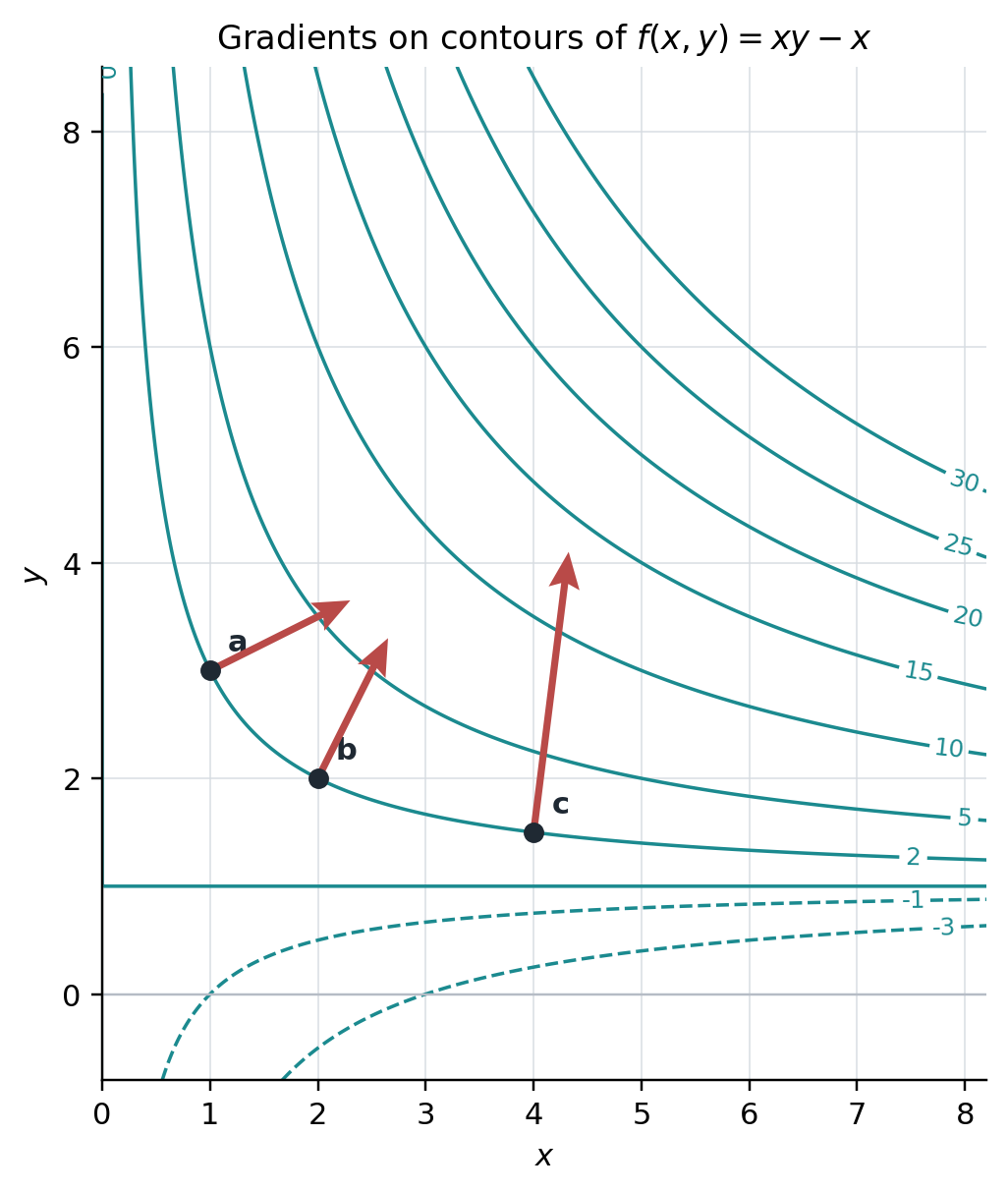
Let \(f(x,y)\) be a function with continuous partial derivatives. If \((a,b)\) is a point where \(\nabla f(a,b) \neq \mathbf{0}\text{,}\) then \(\nabla f(a,b)\) is perpendicular to the level curve of \(f\) passing through the point \((a,b)\text{.}\)
The plot shows level curves of \(f(x,y)=xy-x\) in the first quadrant and slightly below the \(x\)-axis. Three labeled points appear on different level curves: \(\mathbf{a}=(1,3)\text{,}\)\(\mathbf{b}=(2,2)\text{,}\) and \(\mathbf{c}=(4,3/2)\text{.}\) A red arrow begins at each point and points in the direction of the gradient \(\nabla f=(y-1,x)\text{,}\) crossing the nearby contour lines at right angles.
Figure3.3.30.A contour plot of the function \(f(x,y) = xy - x\text{,}\) with the gradient vectors at three points \(\mathbf{a} = (1,3)\text{,}\)\(\mathbf{b} = (2,2)\text{,}\) and \(\mathbf{c} = (4,3/2)\text{.}\) Adapted from: Stanford’s MATH 51 textbook
Let \(f\) be a scalar-valued function of \(n\) variables, and suppose the second partial derivatives of \(f\) exist at a point \(\mathbf{x}\text{.}\) The Hessian matrix of \(f\) at \(\mathbf{x}\) is the \(n \times n\) matrix of second partial derivatives:
That is, \(H_f(\mathbf{x})\) is the matrix whose \((i,j)\)-entry is the second derivative \(\frac{\partial^2 f}{\partial x_i \partial x_j}\) obtained by first differentiating in the \(x_j\) variable, and then the \(x_i\) variable. When the relevant mixed second partial derivatives are continuous on a ball around \(\mathbf{x}\text{,}\) Clairaut’s Theorem implies that the Hessian is symmetric at \(\mathbf{x}\text{.}\)
Next, we compute the second derivatives of \(f\text{.}\) We compute that \(f_{xx} = f_{yy} = f_{zz} = 0\text{,}\) and that \(f_{xy} = f_{xz} = f_{yx} = f_{yz} = f_{zx} = f_{zy} = 1\text{.}\) So
The Jacobian matrix generalizes the concept of the derivative to a vector-valued map of multiple variables. It provides a compact representation of all first-order partial derivatives of a function.