SubsectionLimits and continuity of scalar-valued functions
SubsubsectionBalls, limits, and continuity
This short section supplies local language used in derivative and optimization statements: balls, limits, continuity, interior points, boundary points, closed sets, and bounded sets.
Recall the definition of a limit from single-variable calculus. For a function \(f: \R \to \R\) and \(a,b \in \R\text{,}\) the equation
\begin{equation*}
\lim_{x \to a} f(x) = b
\end{equation*}
holds if for each \(\varepsilon > 0\text{,}\) there is \(\delta > 0\) so that if \(0 \lt |x - a| \lt \delta\text{,}\) then \(|f(x) - b| \lt \varepsilon\text{.}\) We can interpret this statement geometrically as follows: for any open interval \(J\) centered at \(b\text{,}\) there is an open interval \(I\) centered at \(a\) so that \(f\) maps points in \(I\text{,}\) excluding \(a\) itself, into \(J\text{.}\)
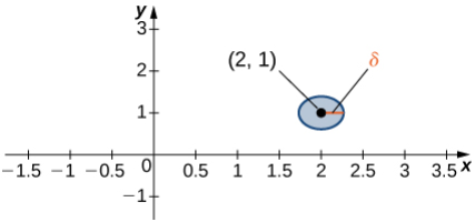
Consider a point \((a,b) \in \mathbb{R}^2\text{.}\) The \(\delta\)-disk centered at point \((a,b)\) is the region of \(\R^2\) bounded by the circle of radius \(\delta\) centered at \((a,b)\text{,}\) i.e., the set
The \(xy\)-plane is shown with a small blue disk centered at the black point \((2,1)\text{.}\) An arrow labeled \(\delta\) points from the center to the edge of the disk, indicating the disk’s radius. The disk lies near the positive \(x\)-axis and above the positive \(y\)-axis tick mark \(1\text{.}\)
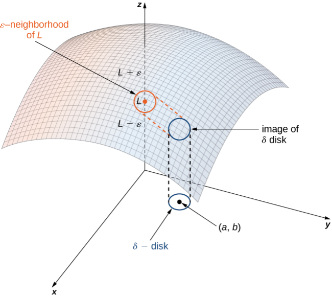
will then hold precisely when, for each open interval \(I\) centered at \(L\text{,}\) there is a \(\delta\) disk centered at \((a,b)\) so that all points in this disk which are also contained in the domain of \(f\text{,}\) excluding the point \((a,b)\) itself, are mapped by \(f\) into \(I\text{.}\)
A 3D surface is drawn above the \(xy\)-plane, with a disk of radius \(\delta\) centered at \((a,b)\) in the domain. A vertical guide from the disk reaches the surface near the height \(L\text{.}\) A shaded band labeled as an \(\varepsilon\)-neighborhood of \(L\) indicates that the image of the disk stays between \(L-\varepsilon\) and \(L+\varepsilon\text{.}\)
Using vector-notation (recalling Definition 1.1.3), we can write a \(\delta\)-disk centered at a point \(\mathbf{x}_0 \in \R^2\) as the set of points \(\mathbf{x} \in \R^2\) so that
if for each \(\varepsilon > 0\text{,}\) there is \(\delta > 0\) so that for any points in the domain of \(f\) with \(0 \lt \| \mathbf{x} - \mathbf{x}_0 \| \lt \delta\text{,}\) the inequality \(|f(\mathbf{x}) - L| \lt \varepsilon\) holds.
In order for the limit of \(f\text{,}\) when it exists, to be unique, the point \(\mathbf{x}_0\) must have the property that the domain of \(f\) contains a point other than \(\mathbf{x}_0\) in any \(\delta\)-ball centered at \(\mathbf{x}_0\text{.}\) This is only a small issue, since every point in the domain of any of the functions that naturally occur in calculus have this property.
Recall from the calculus of a single variable that a function \(f: \R \to \R\) is continuous at a point \(a\) when \(\lim_{x \to a} f(x) = f(a)\text{,}\) i.e., when the limit on the left hand side exists and is equal to the right hand side. The continuity of functions of several variables is defined in exactly the same way.
A scalar-valued function \(f\) is continuous at a point \(\mathbf{x}_0\) in its domain if the limit of \(f\) as \(\mathbf{x} \to \mathbf{x}_0\) exists, and
Definition3.2.9.Interior, boundary, and closed sets.
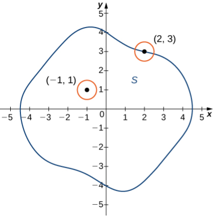
Let \(S\) be a subset of \(\R^n\text{.}\) Then a point \(\mathbf{x}_0 \in S\) is an interior point if there is a \(\delta\)-ball centered at \(\mathbf{x}_0\) completely contained in \(S\text{.}\) A point \(\mathbf{x}_0 \in \R^n\) is a boundary point if every ball centered at \(\mathbf{x}_0\) contains at least one point of \(S\) and at least one point outside \(S\text{.}\) The set of all boundary points of a set \(S\) is called the boundary of the set \(S\text{.}\)
The set \(S\) is drawn as an irregular closed blue curve in the coordinate plane. The point \((-1,1)\) appears inside the curve with a small orange neighborhood around it. The point \((2,3)\) lies on the boundary, and its small orange neighborhood crosses both inside and outside the set.
Note that a boundary point of a set \(S\)need not be contained in the set \(S\). For example, the \(\delta\)-disk defined in this section does not contain its circular boundary. A set that contains its boundary is called closed.
A set \(S \subset \R^n\) is called closed if it contains its boundary. A set \(S \subset \R^n\) is bounded if it is contained in some ball centered at the origin, or equivalently if all points of \(S\) lie within some fixed distance of the origin.