
MATH 345: Linear Algebra and Optimization

Section 7.3 Polynomial spaces and course connections

Sections 7.1 and 7.2 introduced the abstract language. We now use bounded-degree polynomial spaces as a finite-dimensional test world for that language. A polynomial has coefficient coordinates, but the same polynomial space can carry several useful inner products. Changing the inner product changes the projection, so it changes what “best approximation” means.
The goal is not a full theory of polynomial approximation. The goal is to see how vector spaces, inner products, projections, least squares, Taylor approximation, Gram-Schmidt, and Hessians fit together in one concrete setting.

Subsection Polynomials as vectors

A bounded-degree polynomial space is finite-dimensional:
\begin{equation*} \mathcal P_{\le d} = \{a_0+a_1x+\cdots+a_dx^d:a_0,\ldots,a_d\in\mathbb R\}. \end{equation*}
The standard ordered basis is
\begin{equation*} B=(1,x,x^2,\ldots,x^d). \end{equation*}
If
\begin{equation*} p(x)=a_0+a_1x+\cdots+a_dx^d, \end{equation*}
then the coordinate vector of \(p\) in the basis \(B\) is
\begin{equation*} \mathbf c_p = \begin{bmatrix} a_0\\ a_1\\ \vdots\\ a_d \end{bmatrix}. \end{equation*}
The polynomial \(p\) is the vector in \(\mathcal P_{\le d}\text{.}\) The column \(\mathbf c_p\) is its coordinate vector after the basis has been chosen.

Activity 7.3.1. Polynomial coordinates.

Work in \(\mathcal P_{\le3}\) with ordered basis
\begin{equation*} B=(1,x,x^2,x^3). \end{equation*}
Find the coordinate vectors of
\begin{equation*} p(x)=2-3x+x^3,\qquad q(x)=x^2-4x,\qquad r(x)=5. \end{equation*}
Solution.
Match coefficients in the order \(1,x,x^2,x^3\text{:}\)
\begin{equation*} \mathbf c_p= \begin{bmatrix} 2\\ -3\\ 0\\ 1 \end{bmatrix}, \qquad \mathbf c_q= \begin{bmatrix} 0\\ -4\\ 1\\ 0 \end{bmatrix}, \qquad \mathbf c_r= \begin{bmatrix} 5\\ 0\\ 0\\ 0 \end{bmatrix}. \end{equation*}
The degree-at-most-one polynomial space
\begin{equation*} \mathcal P_{\le1}=\operatorname{span}\{1,x\} \end{equation*}
is a subspace of \(\mathcal P_{\le d}\) when \(d\ge1\text{.}\) Its elements have the form
\begin{equation*} c_0+c_1x. \end{equation*}
These are the affine polynomials in one variable. Although the word affine often signals a shifted object, \(\mathcal P_{\le1}\) is a vector subspace: it contains the zero polynomial and is closed under addition and scalar multiplication.

Activity 7.3.2. A root condition as a subspace.

Let
\begin{equation*} U=\{p\in\mathcal P_{\le4}:p(-2)=0\}. \end{equation*}
Explain why \(U\) is a subspace of \(\mathcal P_{\le4}\text{,}\) and find a basis for \(U\text{.}\)
Solution.
The zero polynomial satisfies \(0(-2)=0\text{,}\) so \(0\in U\text{.}\) If \(p(-2)=0\) and \(q(-2)=0\text{,}\) then
\begin{equation*} (p+q)(-2)=p(-2)+q(-2)=0. \end{equation*}
If \(c\in\mathbb R\text{,}\) then
\begin{equation*} (cp)(-2)=c\,p(-2)=0. \end{equation*}
Thus \(U\) is a subspace.
A polynomial satisfies \(p(-2)=0\) exactly when \(x+2\) is a factor. Since \(p\in\mathcal P_{\le4}\text{,}\)
\begin{equation*} p(x)=(x+2)(a_0+a_1x+a_2x^2+a_3x^3). \end{equation*}
Therefore a basis is
\begin{equation*} x+2,\qquad x(x+2),\qquad x^2(x+2),\qquad x^3(x+2). \end{equation*}

Activity 7.3.3. Vanishing value and slope.

Let
\begin{equation*} W=\{p\in\mathcal P_{\le3}:p(0)=0,\ p'(0)=0\}. \end{equation*}
Find a basis for \(W\text{.}\)
Solution.
Write
\begin{equation*} p(x)=a_0+a_1x+a_2x^2+a_3x^3. \end{equation*}
Then
\begin{equation*} p(0)=a_0,\qquad p'(0)=a_1. \end{equation*}
The conditions \(p(0)=0\) and \(p'(0)=0\) force \(a_0=0\) and \(a_1=0\text{.}\) Thus
\begin{equation*} p(x)=a_2x^2+a_3x^3, \end{equation*}
so
\begin{equation*} W=\operatorname{span}\{x^2,x^3\}. \end{equation*}
A basis is \(x^2,x^3\text{.}\)
The next question is not whether \(\mathcal P_{\le1}\) is a subspace. It is: which element of \(\mathcal P_{\le1}\) is closest to a given polynomial or function? That question needs an inner product.

Subsection Inner products and projection equations

The same vector space can carry different inner products. Different inner products give different lengths, distances, orthogonality conditions, and projections.
Let
\begin{equation*} p(x)=a_0+a_1x+\cdots+a_dx^d, \qquad q(x)=b_0+b_1x+\cdots+b_dx^d. \end{equation*}
The coefficient inner product is
\begin{equation*} \langle p,q\rangle_{\mathrm{coef}} = a_0b_0+a_1b_1+\cdots+a_db_d. \end{equation*}
This is the ordinary dot product of the coordinate vectors in the basis \(1,x,\ldots,x^d\text{.}\)
Another useful inner product is the \(L^2[-1,1]\) inner product:
\begin{equation*} \langle p,q\rangle_{L^2} = \int_{-1}^{1}p(x)q(x)\,dx. \end{equation*}
This inner product measures agreement over the whole interval \([-1,1]\text{.}\)
Given sample points \(x_1,\ldots,x_N\text{,}\) the sampled inner product is
\begin{equation*} \langle p,q\rangle_{\mathrm{sample}} = \sum_{i=1}^{N}p(x_i)q(x_i). \end{equation*}
This is the inner product behind sampled least squares and polynomial regression.

Warning 7.3.1.

A sampled rule can fail to be an inner product on all of \(\mathcal P_{\le d}\) if a nonzero polynomial in \(\mathcal P_{\le d}\) vanishes at every sample point. In the computations below, the sample points are chosen so the feature columns in the approximation subspace are independent. That is enough for the least-squares projection used here.
Suppose
\begin{equation*} U=\operatorname{span}\{\phi_0,\phi_1,\ldots,\phi_m\} \end{equation*}
is a polynomial subspace. We want the best approximation to \(f\) inside \(U\text{.}\) Write
\begin{equation*} q=c_0\phi_0+c_1\phi_1+\cdots+c_m\phi_m. \end{equation*}
The residual is
\begin{equation*} r=f-q. \end{equation*}
The projection condition is
\begin{equation*} \langle r,\phi_i\rangle=0, \qquad i=0,\ldots,m. \end{equation*}
Substituting the formula for \(q\) gives
\begin{equation*} \sum_{j=0}^{m}c_j\langle \phi_j,\phi_i\rangle = \langle f,\phi_i\rangle, \qquad i=0,\ldots,m. \end{equation*}
This is the Gram-matrix system
\begin{equation*} G\mathbf c=\mathbf b, \end{equation*}
where
\begin{equation*} G_{ij}=\langle \phi_j,\phi_i\rangle, \qquad b_i=\langle f,\phi_i\rangle, \end{equation*}
and
\begin{equation*} \mathbf c= \begin{bmatrix} c_0\\ c_1\\ \vdots\\ c_m \end{bmatrix}, \qquad \mathbf b= \begin{bmatrix} b_0\\ b_1\\ \vdots\\ b_m \end{bmatrix}. \end{equation*}

Activity 7.3.4. The Gram matrix for affine polynomials.

Let
\begin{equation*} U=\mathcal P_{\le1}=\operatorname{span}\{1,x\} \end{equation*}
with the \(L^2[-1,1]\) inner product. Compute the Gram matrix for the ordered basis
\begin{equation*} \phi_0=1,\qquad \phi_1=x. \end{equation*}
Solution.
We compute
\begin{equation*} \langle 1,1\rangle=\int_{-1}^{1}1\,dx=2, \end{equation*}
\begin{equation*} \langle 1,x\rangle=\int_{-1}^{1}x\,dx=0, \end{equation*}
\begin{equation*} \langle x,1\rangle=\int_{-1}^{1}x\,dx=0, \end{equation*}
and
\begin{equation*} \langle x,x\rangle=\int_{-1}^{1}x^2\,dx=\frac23. \end{equation*}
Thus
\begin{equation*} G= \begin{bmatrix} 2\amp0\\ 0\amp\frac23 \end{bmatrix}. \end{equation*}
If \(q=c_0+c_1x\) is the \(L^2[-1,1]\)-projection of \(f\) onto \(\mathcal P_{\le1}\text{,}\) then
\begin{equation*} \begin{bmatrix} 2\amp0\\ 0\amp\frac23 \end{bmatrix} \begin{bmatrix} c_0\\ c_1 \end{bmatrix} = \begin{bmatrix} \int_{-1}^{1}f(x)\,dx\\ \int_{-1}^{1}xf(x)\,dx \end{bmatrix}. \end{equation*}

Activity 7.3.5. Sampled projection and the design matrix.

Let \(x_1,\ldots,x_N\) be sample points and suppose we approximate sampled values of \(f\) by
\begin{equation*} q(x)=c_0+c_1x. \end{equation*}
Define
\begin{equation*} A= \begin{bmatrix} 1\amp x_1\\ 1\amp x_2\\ \vdots\amp\vdots\\ 1\amp x_N \end{bmatrix}, \qquad \mathbf c= \begin{bmatrix} c_0\\ c_1 \end{bmatrix}, \qquad \mathbf y= \begin{bmatrix} f(x_1)\\ f(x_2)\\ \vdots\\ f(x_N) \end{bmatrix}. \end{equation*}
Explain why the sampled residual condition is
\begin{equation*} A^T\mathbf r=\mathbf{0}, \qquad \mathbf r=\mathbf y-A\mathbf c. \end{equation*}
Solution.
The vector \(A\mathbf c\) stores the fitted values
\begin{equation*} q(x_1),q(x_2),\ldots,q(x_N). \end{equation*}
Thus
\begin{equation*} \mathbf r=\mathbf y-A\mathbf c \end{equation*}
stores the sampled residuals
\begin{equation*} r_i=f(x_i)-q(x_i). \end{equation*}
The sampled projection condition says the residual is orthogonal to the sampled constant feature and the sampled \(x\)-feature:
\begin{equation*} \sum_i r_i=0, \qquad \sum_i x_ir_i=0. \end{equation*}
These are exactly the two entries of
\begin{equation*} A^T\mathbf r= \begin{bmatrix} \sum_i r_i\\ \sum_i x_ir_i \end{bmatrix}. \end{equation*}
So \(A^T\mathbf r=\mathbf{0}\) is the sampled residual-orthogonality condition.

Note 7.3.2.

Polynomial regression is linear regression with polynomial feature columns. For example, fitting
\begin{equation*} y\approx c_0+c_1x+c_2x^2 \end{equation*}
uses the design matrix
\begin{equation*} A= \begin{bmatrix} 1\amp x_1\amp x_1^2\\ 1\amp x_2\amp x_2^2\\ \vdots\amp\vdots\amp\vdots\\ 1\amp x_N\amp x_N^2 \end{bmatrix}. \end{equation*}
The model is nonlinear in \(x\text{,}\) but it is linear in the coefficient vector
\begin{equation*} \mathbf c= \begin{bmatrix} c_0\\ c_1\\ c_2 \end{bmatrix}. \end{equation*}
The next subsection uses one polynomial and one approximation subspace, but three different error measures: local Taylor matching, continuous \(L^2\)-least squares, and sampled least squares.

Subsection Taylor line versus least-squares line

We now use one polynomial and one approximation subspace, but three different meanings of "best".
Let
\begin{equation*} p(x)=1+2x+x^2+x^3, \end{equation*}
and let
\begin{equation*} U=\mathcal P_{\le1}=\operatorname{span}\{1,x\}. \end{equation*}
Every element of \(U\) has the form
\begin{equation*} q(x)=\alpha+\beta x. \end{equation*}
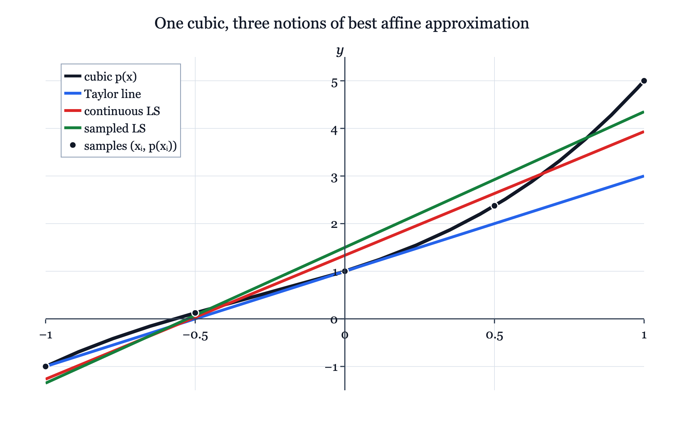
The Taylor line, the continuous least-squares line, and the sampled least-squares line all live in \(U\text{.}\) They differ because they measure error differently.

Activity 7.3.6. Taylor line at the origin.

Find the first-order Taylor approximation to \(p\) at \(0\text{.}\) Then verify the residual conditions.
Solution.
We compute
\begin{equation*} p(0)=1. \end{equation*}
Also
\begin{equation*} p'(x)=2+2x+3x^2, \end{equation*}
so
\begin{equation*} p'(0)=2. \end{equation*}
Thus the first-order Taylor approximation at \(0\) is
\begin{equation*} T(x)=p(0)+p'(0)x=1+2x. \end{equation*}
The residual is
\begin{equation*} r_T(x)=p(x)-T(x)=x^2+x^3. \end{equation*}
Therefore
\begin{equation*} r_T(0)=0, \end{equation*}
and
\begin{equation*} r_T'(x)=2x+3x^2, \end{equation*}
so
\begin{equation*} r_T'(0)=0. \end{equation*}
The Taylor line matches the value and slope of \(p\) at the origin.

Activity 7.3.7. Continuous least-squares line.

Use the \(L^2[-1,1]\) inner product to find the best approximation to \(p\) in \(U=\operatorname{span}\{1,x\}\text{.}\)
Solution.
Write
\begin{equation*} q_{L^2}(x)=\alpha+\beta x. \end{equation*}
The residual is
\begin{equation*} r_{L^2}(x)=p(x)-q_{L^2}(x). \end{equation*}
The projection condition says
\begin{equation*} \langle r_{L^2},1\rangle_{L^2}=0, \qquad \langle r_{L^2},x\rangle_{L^2}=0. \end{equation*}
Equivalently,
\begin{equation*} \int_{-1}^{1}r_{L^2}(x)\,dx=0, \qquad \int_{-1}^{1}x\,r_{L^2}(x)\,dx=0. \end{equation*}
Now
\begin{equation*} r_{L^2}(x) = (1-\alpha)+(2-\beta)x+x^2+x^3. \end{equation*}
The first residual equation gives
\begin{equation*} \int_{-1}^{1}\big((1-\alpha)+(2-\beta)x+x^2+x^3\big)\,dx=0. \end{equation*}
The odd terms integrate to zero on \([-1,1]\text{,}\) so
\begin{equation*} 2(1-\alpha)+\frac23=0. \end{equation*}
Thus
\begin{equation*} \alpha=\frac43. \end{equation*}
The second residual equation gives
\begin{equation*} \int_{-1}^{1}x\big((1-\alpha)+(2-\beta)x+x^2+x^3\big)\,dx=0. \end{equation*}
Again using symmetry,
\begin{equation*} (2-\beta)\frac23+\frac25=0. \end{equation*}
Thus
\begin{equation*} \beta=\frac{13}{5}. \end{equation*}
So the continuous least-squares line is
\begin{equation*} q_{L^2}(x)=\frac43+\frac{13}{5}x. \end{equation*}

Activity 7.3.8. Sampled least-squares line.

Use the sample points
\begin{equation*} -1,\ -\frac12,\ 0,\ \frac12,\ 1 \end{equation*}
to find the sampled least-squares approximation to \(p\) in \(U=\operatorname{span}\{1,x\}\text{.}\)
Solution.
Let the sample points be \(x_1,\ldots,x_5\text{,}\) and write
\begin{equation*} q_{\mathrm{sample}}(x)=\alpha+\beta x. \end{equation*}
The sampled residuals are
\begin{equation*} r_i=p(x_i)-q_{\mathrm{sample}}(x_i). \end{equation*}
The sampled projection condition is
\begin{equation*} \sum_i r_i=0, \qquad \sum_i x_ir_i=0. \end{equation*}
Equivalently, if
\begin{equation*} A= \begin{bmatrix} 1\amp x_1\\ 1\amp x_2\\ \vdots\amp\vdots\\ 1\amp x_5 \end{bmatrix}, \qquad \mathbf r= \begin{bmatrix} r_1\\ r_2\\ \vdots\\ r_5 \end{bmatrix}, \end{equation*}
then
\begin{equation*} A^T\mathbf r=\mathbf{0}. \end{equation*}
For the symmetric sample points,
\begin{equation*} \sum_i x_i=0, \qquad \sum_i x_i^2=\frac52. \end{equation*}
Also
\begin{equation*} \sum_i p(x_i)=\sum_i(1+2x_i+x_i^2+x_i^3)=5+\frac52=\frac{15}{2}, \end{equation*}
so
\begin{equation*} 5\alpha=\frac{15}{2}, \qquad \alpha=\frac32. \end{equation*}
Next,
\begin{equation*} \sum_i x_ip(x_i) = \sum_i(x_i+2x_i^2+x_i^3+x_i^4) = 2\sum_i x_i^2+\sum_i x_i^4. \end{equation*}
Here
\begin{equation*} \sum_i x_i^4=1+\frac1{16}+0+\frac1{16}+1=\frac{17}{8}, \end{equation*}
so
\begin{equation*} \sum_i x_ip(x_i)=5+\frac{17}{8}=\frac{57}{8}. \end{equation*}
The second residual equation gives
\begin{equation*} \beta\sum_i x_i^2=\sum_i x_ip(x_i), \end{equation*}
so
\begin{equation*} \beta\cdot\frac52=\frac{57}{8}, \qquad \beta=\frac{57}{20}. \end{equation*}
Thus the sampled least-squares line is
\begin{equation*} q_{\mathrm{sample}}(x)=\frac32+\frac{57}{20}x. \end{equation*}
The three approximations are
\begin{gather*} T(x)=1+2x,\\ q_{L^2}(x)=\frac43+\frac{13}{5}x,\\ q_{\mathrm{sample}}(x)=\frac32+\frac{57}{20}x. \end{gather*}
They are different because they solve different projection problems.
Approximation How it is chosen Residual condition
Taylor line match value and slope at \(0\) \(r_T(0)=0,\quad r_T'(0)=0\)
Continuous least squares minimize squared error over \([-1,1]\) \(\int_{-1}^{1}r(x)\,dx=0,\quad \int_{-1}^{1}x\,r(x)\,dx=0\)
Sampled least squares minimize squared error at sample points \(\sum_i r_i=0,\quad \sum_i x_ir_i=0\)
One cubic curve with three different best-fit lines.
A black cubic curve is shown on coordinate axes with three colored affine approximations. The blue Taylor line matches the curve near one marked point, the red continuous least-squares line balances error over the interval, and the green sampled least-squares line is influenced by the plotted sample points. The three lines have similar slopes but visibly different positions, showing that the best line depends on the error measure.
Figure 7.3.3. One curve, three lines: Taylor, continuous least squares, and sampled least squares measure best approximation differently.

Warning 7.3.4.

The phrase “best affine approximation” is incomplete until the error measure is specified. Taylor matching, continuous least squares, and sampled least squares give different answers because they use different residual conditions.
The next subsection explains how Taylor approximation itself can be viewed as projection, but with a local derivative-based inner product.

Subsection Taylor approximation as local projection

The previous subsection showed that Taylor and least squares can give different lines. This is not a contradiction. Taylor approximation is local. Ordinary \(L^2\)-least squares over a fixed interval is global.
There are two useful ways to connect Taylor approximation with projection.
First, Taylor approximation is exactly projection for a derivative-based inner product at the expansion point.
Second, ordinary \(L^2\)-least-squares projection over a shrinking interval converges to Taylor approximation as the interval shrinks to the expansion point.
Derivative-based inner product. Fix a point \(a\text{,}\) and work in \(\mathcal P_{\le d}\text{.}\) Define
\begin{equation*} \langle p,q\rangle_{\mathrm{jet},a} = \sum_{k=0}^{d} w_k \frac{p^{(k)}(a)}{k!} \frac{q^{(k)}(a)}{k!}, \qquad w_k>0. \end{equation*}
This is an inner product on \(\mathcal P_{\le d}\text{,}\) because a polynomial of degree at most \(d\) is determined by its derivatives through order \(d\) at \(a\text{.}\)

Activity 7.3.9. Taylor line as exact projection.

Suppose
\begin{equation*} p(x)=c_0+c_1(x-a)+c_2(x-a)^2+c_3(x-a)^3 \end{equation*}
and let
\begin{equation*} q(x)=\alpha+\beta(x-a). \end{equation*}
Use the derivative-based inner product above to find the closest affine polynomial \(q\) to \(p\text{.}\)
Solution.
In the centered basis
\begin{equation*} 1,\quad (x-a),\quad (x-a)^2,\quad (x-a)^3, \end{equation*}
the coefficients of \(p\) are \(c_0,c_1,c_2,c_3\text{,}\) while the coefficients of \(q\) are \(\alpha,\beta,0,0\text{.}\) Therefore
\begin{equation*} p-q=(c_0-\alpha)+(c_1-\beta)(x-a)+c_2(x-a)^2+c_3(x-a)^3. \end{equation*}
The squared norm of the residual has the form
\begin{equation*} \|p-q\|_{\mathrm{jet},a}^2 = w_0(c_0-\alpha)^2 + w_1(c_1-\beta)^2 + w_2c_2^2 + w_3c_3^2. \end{equation*}
The last two terms do not depend on \(\alpha\) or \(\beta\text{.}\) The expression is minimized when
\begin{equation*} \alpha=c_0, \qquad \beta=c_1. \end{equation*}
Thus the closest affine polynomial is
\begin{equation*} q(x)=c_0+c_1(x-a). \end{equation*}
Since
\begin{equation*} c_0=p(a), \qquad c_1=p'(a), \end{equation*}
we get
\begin{equation*} q(x)=p(a)+p'(a)(x-a). \end{equation*}
This is the first-order Taylor approximation at \(a\text{.}\)
More generally, projection onto \(\mathcal P_{\le m}\text{,}\) written in powers of \(x-a\text{,}\) keeps the Taylor terms through degree \(m\) and discards the higher-degree terms.

Warning 7.3.5.

The inner product \(\langle\cdot,\cdot\rangle_{\mathrm{jet},a}\) depends on the expansion point \(a\text{.}\) One fixed projection cannot produce the Taylor line at every point, because the Taylor line of the same polynomial changes when the expansion point changes.

Activity 7.3.10. Fixed-interval least squares is not Taylor approximation.

Project
\begin{equation*} p(x)=x^2 \end{equation*}
onto \(\mathcal P_{\le1}=\operatorname{span}\{1,x\}\) using the \(L^2[-1,1]\) inner product. Compare the answer with the Taylor line at \(0\text{.}\)
Solution.
The Taylor line of \(x^2\) at \(0\) is
\begin{equation*} T(x)=0. \end{equation*}
Now compute the \(L^2[-1,1]\)-projection. Write
\begin{equation*} q(x)=\alpha+\beta x. \end{equation*}
Since \(x^2\) is even and \(x\) is odd, the best line has no \(x\)-term:
\begin{equation*} \beta=0. \end{equation*}
The constant term is the average value of \(x^2\) over \([-1,1]\text{:}\)
\begin{equation*} \alpha = \frac{\int_{-1}^{1}x^2\,dx}{\int_{-1}^{1}1\,dx} = \frac{2/3}{2} = \frac13. \end{equation*}
Thus the \(L^2[-1,1]\)-best affine approximation is
\begin{equation*} q(x)=\frac13, \end{equation*}
not \(0\text{.}\) Taylor approximation is local, while least squares over a fixed interval is global.
Shrinking intervals. For \(t>0\text{,}\) let \(P_t f\) be the \(L^2[-t,t]\)-projection of \(f\) onto \(\operatorname{span}\{1,x\}\text{.}\) Write
\begin{equation*} P_t f(x)=a_t+b_t x. \end{equation*}
The residual conditions are
\begin{equation*} \int_{-t}^{t}\big(f(x)-a_t-b_t x\big)\,dx=0, \end{equation*}
and
\begin{equation*} \int_{-t}^{t}x\big(f(x)-a_t-b_t x\big)\,dx=0. \end{equation*}
Because the interval is symmetric,
\begin{equation*} \int_{-t}^{t}x\,dx=0. \end{equation*}
Thus the formulas simplify to
\begin{equation*} a_t=\frac{1}{2t}\int_{-t}^{t}f(x)\,dx, \end{equation*}
and
\begin{equation*} b_t= \frac{\int_{-t}^{t}xf(x)\,dx}{\int_{-t}^{t}x^2\,dx} = \frac{3}{2t^3}\int_{-t}^{t}xf(x)\,dx. \end{equation*}

Activity 7.3.11. Shrinking least squares for \(x^2\) and \(x^3\).

Compute the \(L^2[-t,t]\)-projection of \(x^2\) and \(x^3\) onto \(\operatorname{span}\{1,x\}\text{.}\) What happens as \(t\to0\text{?}\)
Solution.
For \(f(x)=x^2\text{,}\) symmetry gives \(b_t=0\text{,}\) and
\begin{equation*} a_t= \frac{1}{2t}\int_{-t}^{t}x^2\,dx = \frac{1}{2t}\cdot\frac{2t^3}{3} = \frac{t^2}{3}. \end{equation*}
Thus
\begin{equation*} P_t(x^2)=\frac{t^2}{3}. \end{equation*}
As \(t\to0\text{,}\)
\begin{equation*} P_t(x^2)\to0, \end{equation*}
which is the Taylor line of \(x^2\) at \(0\text{.}\)
For \(f(x)=x^3\text{,}\) symmetry gives \(a_t=0\text{,}\) and
\begin{equation*} b_t= \frac{\int_{-t}^{t}x^4\,dx}{\int_{-t}^{t}x^2\,dx} = \frac{2t^5/5}{2t^3/3} = \frac{3t^2}{5}. \end{equation*}
Thus
\begin{equation*} P_t(x^3)=\frac{3t^2}{5}x. \end{equation*}
As \(t\to0\text{,}\)
\begin{equation*} P_t(x^3)\to0, \end{equation*}
which is again the Taylor line at \(0\text{.}\)

Note 7.3.6.

If
\begin{equation*} p(x)=c_0+c_1x+c_2x^2+\cdots+c_dx^d, \end{equation*}
then the \(L^2[-t,t]\)-projection of \(p\) onto \(\operatorname{span}\{1,x\}\) has the form
\begin{equation*} P_t p(x)=a_t+b_t x, \end{equation*}
where
\begin{equation*} a_t = c_0+\frac{c_2t^2}{3}+\frac{c_4t^4}{5}+\frac{c_6t^6}{7}+\cdots \end{equation*}
and
\begin{equation*} b_t = c_1+\frac{3c_3t^2}{5}+\frac{3c_5t^4}{7}+\frac{3c_7t^6}{9}+\cdots. \end{equation*}
Therefore
\begin{equation*} a_t\to c_0=p(0), \qquad b_t\to c_1=p'(0). \end{equation*}
So
\begin{equation*} P_t p(x)\to p(0)+p'(0)x. \end{equation*}
This is the first-order Taylor polynomial at \(0\text{.}\)

Warning 7.3.7.

The projections \(P_t p\) can converge to Taylor approximation even though the inner products collapse as \(t\to0\text{.}\) In fact, for
\begin{equation*} \langle p,q\rangle_t=\int_{-t}^{t}p(x)q(x)\,dx, \end{equation*}
we have
\begin{equation*} \langle p,q\rangle_t\to0 \end{equation*}
for fixed polynomials \(p,q\text{.}\) If we normalize by interval length, the limit only remembers the value at the origin:
\begin{equation*} \frac{1}{2t}\int_{-t}^{t}p(x)q(x)\,dx\to p(0)q(0). \end{equation*}
That is not a nondegenerate inner product on \(\mathcal P_{\le d}\text{.}\) The Taylor-coefficient inner product appears only after separating degrees by scale. For this course, the important point is: shrinking \(L^2\)-projections recover Taylor polynomials, but the ordinary \(L^2[-t,t]\) inner products themselves do not converge to the derivative-based Taylor inner product.
The single-variable picture is now complete:
\begin{gather*} \text{fixed-interval least squares is global,}\\ \text{shrinking-interval least squares becomes local,}\\ \text{the derivative-based inner product makes Taylor projection exact.} \end{gather*}

Subsection Gram-Schmidt and Legendre polynomials

Gram-Schmidt is not only an algorithm for column vectors in \(\mathbb R^n\text{.}\) It works in any finite-dimensional inner product space. Here the vectors are polynomials.
Use the inner product
\begin{equation*} \langle f,g\rangle = \int_{-1}^{1}f(x)g(x)\,dx \end{equation*}
on \(\mathcal P_{\le3}\text{.}\) Start with the standard ordered basis
\begin{equation*} 1,\quad x,\quad x^2,\quad x^3. \end{equation*}
This basis spans \(\mathcal P_{\le3}\text{,}\) but it is not an orthogonal basis. Gram-Schmidt replaces it with an orthogonal basis for the same polynomial space.

Note 7.3.8. Symmetry on \([-1,1]\).

If \(h(x)\) is an odd function, then
\begin{equation*} \int_{-1}^{1}h(x)\,dx=0. \end{equation*}
This explains many zeros below. Products with odd total power integrate to zero on the symmetric interval.

Activity 7.3.12. The first two orthogonal polynomials.

Show that \(1\) and \(x\) are orthogonal using the \(L^2[-1,1]\) inner product.
Solution.
We compute
\begin{equation*} \langle 1,x\rangle = \int_{-1}^{1}x\,dx = 0. \end{equation*}
Thus \(1\) and \(x\) are already orthogonal.

Activity 7.3.13. Orthogonalizing \(x^2\).

Let
\begin{equation*} \phi_0(x)=1, \qquad \phi_1(x)=x. \end{equation*}
Use Gram-Schmidt to subtract from \(x^2\) its projections onto \(\phi_0\) and \(\phi_1\text{.}\)
Solution.
First,
\begin{equation*} \langle x^2,1\rangle = \int_{-1}^{1}x^2\,dx = \frac23, \end{equation*}
and
\begin{equation*} \langle 1,1\rangle = \int_{-1}^{1}1\,dx = 2. \end{equation*}
Therefore
\begin{equation*} \operatorname{proj}_{\operatorname{span}\{1\}}(x^2) = \frac{\langle x^2,1\rangle}{\langle 1,1\rangle}1 = \frac{2/3}{2}1 = \frac13. \end{equation*}
Also,
\begin{equation*} \langle x^2,x\rangle = \int_{-1}^{1}x^3\,dx = 0, \end{equation*}
so there is no \(x\)-component to subtract. Thus the next orthogonal vector is
\begin{equation*} \phi_2(x)=x^2-\frac13. \end{equation*}

Activity 7.3.14. Orthogonalizing \(x^3\).

Let
\begin{equation*} \phi_0(x)=1, \qquad \phi_1(x)=x, \qquad \phi_2(x)=x^2-\frac13. \end{equation*}
Use Gram-Schmidt to subtract from \(x^3\) its projections onto \(\phi_0,\phi_1,\phi_2\text{.}\)
Solution.
By symmetry,
\begin{equation*} \langle x^3,1\rangle = \int_{-1}^{1}x^3\,dx = 0. \end{equation*}
Also,
\begin{equation*} \langle x^3,\phi_2\rangle = \int_{-1}^{1}x^3\left(x^2-\frac13\right)\,dx = \int_{-1}^{1}\left(x^5-\frac13x^3\right)\,dx = 0, \end{equation*}
again by symmetry.
The only projection to subtract is the projection onto \(x\text{.}\) We compute
\begin{equation*} \langle x^3,x\rangle = \int_{-1}^{1}x^4\,dx = \frac25, \end{equation*}
and
\begin{equation*} \langle x,x\rangle = \int_{-1}^{1}x^2\,dx = \frac23. \end{equation*}
Thus
\begin{equation*} \operatorname{proj}_{\operatorname{span}\{x\}}(x^3) = \frac{\langle x^3,x\rangle}{\langle x,x\rangle}x = \frac{2/5}{2/3}x = \frac35x. \end{equation*}
Therefore the next orthogonal vector is
\begin{equation*} \phi_3(x)=x^3-\frac35x. \end{equation*}
Gram-Schmidt has produced the orthogonal basis
\begin{equation*} 1,\qquad x,\qquad x^2-\frac13,\qquad x^3-\frac35x \end{equation*}
for \(\mathcal P_{\le3}\text{,}\) using the \(L^2[-1,1]\) inner product.

Warning 7.3.9. Orthogonal does not mean normalized.

The vectors above are orthogonal, but their norms are not all equal to \(1\text{.}\) Gram-Schmidt can produce an orthogonal basis first; normalizing each vector is a separate step.

Note 7.3.10. Scaled Legendre polynomials.

The conventional first Legendre polynomials begin
\begin{equation*} P_0(x)=1, \qquad P_1(x)=x, \end{equation*}
\begin{equation*} P_2(x)=\frac12(3x^2-1), \qquad P_3(x)=\frac12(5x^3-3x). \end{equation*}
These are nonzero scalar multiples of
\begin{equation*} 1,\qquad x,\qquad x^2-\frac13,\qquad x^3-\frac35x. \end{equation*}
We do not develop the theory of Legendre polynomials here. The point is that Gram-Schmidt creates coordinates adapted to an inner product.
When \(\phi_0,\ldots,\phi_m\) are nonzero and orthogonal, projection onto
\begin{equation*} U=\operatorname{span}\{\phi_0,\ldots,\phi_m\} \end{equation*}
has the simple form
\begin{equation*} \operatorname{proj}_U(f) = \sum_{j=0}^{m} \frac{\langle f,\phi_j\rangle}{\langle \phi_j,\phi_j\rangle}\phi_j. \end{equation*}
The Gram matrix is diagonal in an orthogonal basis, so the projection equations decouple.

Activity 7.3.15. Revisiting the continuous least-squares line.

Let
\begin{equation*} p(x)=1+2x+x^2+x^3. \end{equation*}
Use the orthogonal basis
\begin{equation*} \phi_0=1,\qquad \phi_1=x,\qquad \phi_2=x^2-\frac13,\qquad \phi_3=x^3-\frac35x \end{equation*}
to express \(p\text{.}\) Then project \(p\) onto
\begin{equation*} \mathcal P_{\le1}=\operatorname{span}\{1,x\}. \end{equation*}
Solution.
Since
\begin{equation*} x^2=\phi_2+\frac13\phi_0 \end{equation*}
and
\begin{equation*} x^3=\phi_3+\frac35\phi_1, \end{equation*}
we have
\begin{equation*} p(x) = 1+2x+x^2+x^3 \end{equation*}
\begin{equation*} = 1+2\phi_1+\left(\phi_2+\frac13\phi_0\right) + \left(\phi_3+\frac35\phi_1\right). \end{equation*}
Thus
\begin{equation*} p = \frac43\phi_0+\frac{13}{5}\phi_1+\phi_2+\phi_3. \end{equation*}
Projection onto \(\mathcal P_{\le1}=\operatorname{span}\{\phi_0,\phi_1\}\) keeps only the \(\phi_0\) and \(\phi_1\) components:
\begin{equation*} \operatorname{proj}_{\mathcal P_{\le1}}(p) = \frac43\phi_0+\frac{13}{5}\phi_1. \end{equation*}
Since \(\phi_0=1\) and \(\phi_1=x\text{,}\)
\begin{equation*} \operatorname{proj}_{\mathcal P_{\le1}}(p) = \frac43+\frac{13}{5}x. \end{equation*}
This is the continuous least-squares line from the earlier subsection.
The same idea explains why orthogonal bases and QR are useful in least squares: changing to an orthogonal basis does not change the approximation space, but it makes projection computations easier.
The next subsections move from one-variable polynomials to two-variable polynomial spaces. There, affine approximations are planes and quadratic terms are controlled by Hessians.

Subsection Two-variable polynomials and tangent planes

The same ideas work for polynomials in more than one input variable. This is the bridge back to multivariable calculus: affine approximations become planes, sampled least squares becomes plane fitting, and quadratic terms lead to Hessians.
The space of two-variable polynomials of total degree at most \(2\) is
\begin{equation*} \mathcal P_{\le2}^{(2)} = \operatorname{span}\{1,x,y,x^2,xy,y^2\}. \end{equation*}
A standard ordered basis is
\begin{equation*} B=(1,x,y,x^2,xy,y^2). \end{equation*}
An element of \(\mathcal P_{\le2}^{(2)}\) has the form
\begin{equation*} a_0+a_1x+a_2y+a_3x^2+a_4xy+a_5y^2. \end{equation*}
Its coordinate vector in the basis \(B\) is
\begin{equation*} \begin{bmatrix} a_0\\ a_1\\ a_2\\ a_3\\ a_4\\ a_5 \end{bmatrix}. \end{equation*}

Activity 7.3.16. Coordinates in a two-variable polynomial space.

Work in \(\mathcal P_{\le2}^{(2)}\) with ordered basis
\begin{equation*} B=(1,x,y,x^2,xy,y^2). \end{equation*}
Find the coordinate vector of
\begin{equation*} p(x,y)=3-2x+y+5xy. \end{equation*}
Solution.
Match coefficients in the order \(1,x,y,x^2,xy,y^2\text{.}\) We get
\begin{equation*} \mathbf c_p = \begin{bmatrix} 3\\ -2\\ 1\\ 0\\ 5\\ 0 \end{bmatrix}. \end{equation*}
The affine-polynomial subspace is
\begin{equation*} \mathcal A=\operatorname{span}\{1,x,y\}. \end{equation*}
Its elements have the form
\begin{equation*} q(x,y)=\alpha+\beta x+\gamma y. \end{equation*}
Geometrically, the graph of \(q\) is a plane.
Now consider
\begin{equation*} f(x,y)=1+2x-y+x^2+xy+2y^2+x^3. \end{equation*}
At \((0,0)\text{,}\) the tangent plane uses only the value and first partial derivatives of \(f\text{.}\)

Activity 7.3.17. Tangent plane at the origin.

Compute the tangent plane to
\begin{equation*} f(x,y)=1+2x-y+x^2+xy+2y^2+x^3 \end{equation*}
at \((0,0)\text{.}\) Then state the residual conditions it satisfies.
Solution.
We compute
\begin{equation*} f(0,0)=1. \end{equation*}
Also
\begin{equation*} f_x(x,y)=2+2x+y+3x^2, \end{equation*}
so
\begin{equation*} f_x(0,0)=2. \end{equation*}
And
\begin{equation*} f_y(x,y)=-1+x+4y, \end{equation*}
so
\begin{equation*} f_y(0,0)=-1. \end{equation*}
Therefore the tangent plane is
\begin{equation*} T(x,y)=1+2x-y. \end{equation*}
The residual is
\begin{equation*} r_T(x,y)=f(x,y)-T(x,y)=x^2+xy+2y^2+x^3. \end{equation*}
Thus
\begin{equation*} r_T(0,0)=0, \end{equation*}
and
\begin{equation*} \nabla r_T(0,0) = \begin{bmatrix} 0\\ 0 \end{bmatrix}. \end{equation*}
The tangent plane matches the value and first partial derivatives at the origin.
A best-fit plane uses a different idea. Instead of matching at one point, it minimizes error over many points.
Let
\begin{equation*} (x_1,y_1),\ldots,(x_N,y_N) \end{equation*}
be sampled points. Define the sampled inner product by
\begin{equation*} \langle u,v\rangle_{\mathrm{sample}} = \sum_{i=1}^{N}u(x_i,y_i)v(x_i,y_i). \end{equation*}
For a plane
\begin{equation*} q(x,y)=\alpha+\beta x+\gamma y, \end{equation*}
the sampled residuals are
\begin{equation*} r_i=f(x_i,y_i)-q(x_i,y_i). \end{equation*}
The sampled projection conditions are
\begin{equation*} \sum_i r_i=0, \qquad \sum_i x_ir_i=0, \qquad \sum_i y_ir_i=0. \end{equation*}

Activity 7.3.18. Design matrix for a sampled best-fit plane.

Let
\begin{equation*} q(x,y)=\alpha+\beta x+\gamma y. \end{equation*}
Construct the design matrix for fitting \(q\) to sampled values of \(f\) at points
\begin{equation*} (x_1,y_1),\ldots,(x_N,y_N). \end{equation*}
Explain the residual condition in matrix form.
Solution.
The design matrix is
\begin{equation*} A= \begin{bmatrix} 1\amp x_1\amp y_1\\ 1\amp x_2\amp y_2\\ \vdots\amp\vdots\amp\vdots\\ 1\amp x_N\amp y_N \end{bmatrix}. \end{equation*}
The coefficient vector is
\begin{equation*} \mathbf c= \begin{bmatrix} \alpha\\ \beta\\ \gamma \end{bmatrix}, \end{equation*}
and the sampled-value vector is
\begin{equation*} \mathbf f= \begin{bmatrix} f(x_1,y_1)\\ f(x_2,y_2)\\ \vdots\\ f(x_N,y_N) \end{bmatrix}. \end{equation*}
The fitted values are \(A\mathbf c\text{,}\) so the residual vector is
\begin{equation*} \mathbf r=\mathbf f-A\mathbf c. \end{equation*}
The sampled residual-orthogonality condition is
\begin{equation*} A^T\mathbf r=\mathbf{0}. \end{equation*}
Written entry by entry, this says
\begin{equation*} \sum_i r_i=0, \qquad \sum_i x_ir_i=0, \qquad \sum_i y_ir_i=0. \end{equation*}
These are the same projection conditions as before, now for the sampled constant feature, sampled \(x\)-feature, and sampled \(y\)-feature.

Activity 7.3.19. A sampled best-fit plane on a symmetric grid.

Use the grid
\begin{equation*} x,y\in\left\{-1,-\frac12,0,\frac12,1\right\} \end{equation*}
and the function
\begin{equation*} f(x,y)=1+2x-y+x^2+xy+2y^2+x^3. \end{equation*}
Find the sampled least-squares plane
\begin{equation*} q_{\mathrm{sample}}(x,y)=\alpha+\beta x+\gamma y. \end{equation*}
Solution.
The grid has \(25\) points. By symmetry,
\begin{equation*} \sum_i x_i=0, \qquad \sum_i y_i=0, \qquad \sum_i x_iy_i=0. \end{equation*}
Also
\begin{equation*} \sum_i x_i^2=\sum_i y_i^2=\frac{25}{2}, \end{equation*}
and
\begin{equation*} \sum_i x_i^4=\frac{85}{8}. \end{equation*}
Because the grid is symmetric, the normal equations decouple. For the constant term,
\begin{equation*} 25\alpha=\sum_i f(x_i,y_i). \end{equation*}
All odd terms have zero sum on the symmetric grid, and the \(xy\) term also has zero sum. Thus
\begin{equation*} \sum_i f(x_i,y_i) = 25+\sum_i x_i^2+2\sum_i y_i^2 = 25+\frac{25}{2}+25 = \frac{125}{2}. \end{equation*}
Therefore
\begin{equation*} \alpha=\frac52. \end{equation*}
For the \(x\)-coefficient,
\begin{equation*} \beta\sum_i x_i^2=\sum_i x_if(x_i,y_i). \end{equation*}
By symmetry,
\begin{equation*} \sum_i x_if(x_i,y_i) = 2\sum_i x_i^2+\sum_i x_i^4 = 25+\frac{85}{8} = \frac{285}{8}. \end{equation*}
Thus
\begin{equation*} \beta\cdot\frac{25}{2}=\frac{285}{8}, \end{equation*}
so
\begin{equation*} \beta=\frac{57}{20}. \end{equation*}
For the \(y\)-coefficient,
\begin{equation*} \gamma\sum_i y_i^2=\sum_i y_if(x_i,y_i). \end{equation*}
By symmetry, the only surviving term is \(-y\text{,}\) so
\begin{equation*} \sum_i y_if(x_i,y_i)=-\sum_i y_i^2. \end{equation*}
Therefore
\begin{equation*} \gamma=-1. \end{equation*}
The sampled best-fit plane is
\begin{equation*} q_{\mathrm{sample}}(x,y)=\frac52+\frac{57}{20}x-y. \end{equation*}
The tangent plane and sampled best-fit plane are different:
\begin{equation*} T(x,y)=1+2x-y, \end{equation*}
while
\begin{equation*} q_{\mathrm{sample}}(x,y)=\frac52+\frac{57}{20}x-y. \end{equation*}

They are different because they solve different approximation problems.
Plane How it is chosen Residual condition
Tangent plane match value and first partial derivatives at \((0,0)\) \(r(0,0)=0,\quad \nabla r(0,0)=\mathbf{0}\)
Sampled best-fit plane minimize squared error on sampled points \(\sum_i r_i=0,\quad \sum_i x_ir_i=0,\quad \sum_i y_ir_i=0\)
Continuous best-fit plane minimize squared error over a region \(\iint_R r\,dA=0,\quad \iint_R xr\,dA=0,\quad \iint_R yr\,dA=0\)
A curved surface with a local tangent plane and a sampled best-fit plane.
A blue curved surface is shown above a green sampled best-fit plane and a smaller blue tangent plane. The tangent plane touches the surface near a purple tangent point with short purple derivative markers. Several black sample points are scattered across the surface, illustrating that the green plane balances errors over the grid rather than matching one point exactly.
Figure 7.3.11. Tangent plane and sampled best-fit plane for the same surface. The tangent plane is local; the best-fit plane depends on the sampled error measure.

Warning 7.3.12.

A tangent plane is local. A sampled best-fit plane depends on the chosen sample points. A continuous best-fit plane depends on the chosen region and uses double integrals.

Note 7.3.13. Continuous best fit as a preview.

In one variable, the continuous inner product
\begin{equation*} \langle u,v\rangle=\int_{-1}^{1}u(x)v(x)\,dx \end{equation*}
measures agreement over an interval. In two variables, the analogous continuous inner product over a region \(R\) is
\begin{equation*} \langle u,v\rangle_R=\iint_R u(x,y)v(x,y)\,dA. \end{equation*}
MATH 345 does not develop double integrals, so the course-level computation uses sampled sums:
\begin{equation*} \langle u,v\rangle_{\mathrm{sample}} = \sum_i u(x_i,y_i)v(x_i,y_i). \end{equation*}
With many well-spread sample points, a scaled sampled sum can approximate a continuous integral. This is also a bridge to probability: averages over sampled points approximate expected values.
For the square
\begin{equation*} R=[-1,1]\times[-1,1], \end{equation*}
the continuous \(L^2(R)\)-best-fit plane for the same function is
\begin{equation*} q_{L^2}(x,y)=2+\frac{13}{5}x-y. \end{equation*}
This is shown only as a preview. The sampled plane above is the computation used in this course.

Note 7.3.14. Looking ahead.

Students who want to study probability together with the multivariate-integration tools behind continuous averaging can look at UW-Madison MATH 331. The UW Mathematics probability courses page describes MATH 331 as an introductory probability course for students who have not taken multivariable calculus and says it introduces the needed tools from multivariate integration alongside probability: UW-Madison Mathematics probability courses
 1 
www.math.wisc.edu/undergraduate/courses-enrollment/probability-courses/
.
The next subsection keeps the same function and looks at the quadratic terms. Those terms are controlled by the Hessian.

Subsection Hessians as quadratic forms

The previous subsection compared tangent planes with best-fit planes. A tangent plane is the first-order local polynomial model. The next local model keeps the quadratic terms too.
Let
\begin{equation*} \mathbf h= \begin{bmatrix}x\\y\end{bmatrix} \end{equation*}
At the origin, the second-order Taylor polynomial has the form
\begin{equation*} T_2(\mathbf h) = f(\mathbf0) + \nabla f(\mathbf0)\cdot \mathbf h +\frac12 \mathbf h^T H_f(\mathbf0)\mathbf h. \end{equation*}
Here \(H_f(\mathbf0)\) is the Hessian matrix:
\begin{equation*} H_f(\mathbf0) = \begin{bmatrix} f_{xx}(\mathbf0)&f_{xy}(\mathbf0)\\ f_{yx}(\mathbf0)&f_{yy}(\mathbf0) \end{bmatrix}. \end{equation*}
The expression
\begin{equation*} \frac12\mathbf h^T H_f(\mathbf0)\mathbf h \end{equation*}
is the quadratic part of the local polynomial model.

Activity 7.3.20. First- and second-order Taylor polynomials.

Let
\begin{equation*} f(x,y)=1+2x-y+x^2+xy+2y^2+x^3. \end{equation*}
Find the first-order and second-order Taylor polynomials of \(f\) at \((0,0)\text{.}\)
Solution.
From the previous subsection,
\begin{equation*} f(0,0)=1, \qquad f_x(0,0)=2, \qquad f_y(0,0)=-1. \end{equation*}
Thus the first-order Taylor polynomial is
\begin{equation*} T_1(x,y)=1+2x-y. \end{equation*}
The terms of degree at most \(2\) in the polynomial \(f\) are
\begin{equation*} 1+2x-y+x^2+xy+2y^2. \end{equation*}
Therefore the second-order Taylor polynomial at the origin is
\begin{equation*} T_2(x,y)=1+2x-y+x^2+xy+2y^2. \end{equation*}
The residual after the second-order approximation is
\begin{equation*} f(x,y)-T_2(x,y)=x^3. \end{equation*}
This residual has no constant, linear, or quadratic terms at the origin.

Activity 7.3.21. The Hessian as the matrix of the quadratic part.

For
\begin{equation*} f(x,y)=1+2x-y+x^2+xy+2y^2+x^3, \end{equation*}
compute \(H_f(\mathbf0)\text{.}\) Then verify that
\begin{equation*} \frac12\mathbf h^T H_f(\mathbf0)\mathbf h \end{equation*}
is the quadratic part of \(T_2\text{.}\)
Solution.
First compute the second partial derivatives:
\begin{equation*} f_{xx}(x,y)=2+6x, \qquad f_{xy}(x,y)=1, \end{equation*}
\begin{equation*} f_{yx}(x,y)=1, \qquad f_{yy}(x,y)=4. \end{equation*}
At the origin,
\begin{equation*} H_f(\mathbf0) = \begin{bmatrix} 2&1\\ 1&4 \end{bmatrix}. \end{equation*}
Now
\begin{equation*} \frac12\mathbf h^T H_f(\mathbf0)\mathbf h = \frac12 \begin{bmatrix}x&y\end{bmatrix} \begin{bmatrix} 2&1\\ 1&4 \end{bmatrix} \begin{bmatrix}x\\y\end{bmatrix}. \end{equation*}
Multiplying gives
\begin{equation*} \begin{bmatrix} 2&1\\ 1&4 \end{bmatrix} \begin{bmatrix}x\\y\end{bmatrix} = \begin{bmatrix} 2x+y\\ x+4y \end{bmatrix}, \end{equation*}
so
\begin{equation*} \frac12 \begin{bmatrix}x&y\end{bmatrix} \begin{bmatrix} 2x+y\\ x+4y \end{bmatrix} = \frac12(2x^2+2xy+4y^2). \end{equation*}
Therefore
\begin{equation*} \frac12\mathbf h^T H_f(\mathbf0)\mathbf h = x^2+xy+2y^2. \end{equation*}
This is exactly the quadratic part of
\begin{equation*} T_2(x,y)=1+2x-y+x^2+xy+2y^2. \end{equation*}

Warning 7.3.15.

The Hessian does not contain the constant term or the linear term. It only records the quadratic part of the local polynomial model. The factor \(\frac12\) appears because the symmetric matrix contributes the mixed term twice:
\begin{equation*} \begin{bmatrix}x&y\end{bmatrix} \begin{bmatrix} 0&1\\ 1&0 \end{bmatrix} \begin{bmatrix}x\\y\end{bmatrix} = 2xy. \end{equation*}

Activity 7.3.22. Reading the sign of a quadratic form.

Let
\begin{equation*} Q(\mathbf h)=\frac12\mathbf h^T \begin{bmatrix} 2&1\\ 1&4 \end{bmatrix} \mathbf h. \end{equation*}
Show that \(Q(\mathbf h)>0\) for every nonzero vector \(\mathbf h\text{.}\) What would this mean at a critical point?
Solution.
From the previous activity,
\begin{equation*} Q(\mathbf h)=x^2+xy+2y^2. \end{equation*}
Complete the square:
\begin{equation*} x^2+xy+2y^2 = \left(x+\frac12y\right)^2+\frac74y^2. \end{equation*}
Both terms on the right are nonnegative, and they are both zero only when
\begin{equation*} y=0 \end{equation*}
and then
\begin{equation*} x=0. \end{equation*}
Thus
\begin{equation*} Q(\mathbf h)>0 \end{equation*}
for every nonzero
\begin{equation*} \mathbf h= \begin{bmatrix}x\\y\end{bmatrix}. \end{equation*}
If this quadratic form appeared at a critical point, then the second-order local model would curve upward in every nonzero direction. This is the positive-definite case in the second derivative test, so the critical point would be a local minimum.

Note 7.3.16.

In our running example,
\begin{equation*} \nabla f(\mathbf0)= \begin{bmatrix} 2\\ -1 \end{bmatrix}, \end{equation*}
so the origin is not a critical point. The positive quadratic part describes curvature, but it does not make \((0,0)\) a local minimum because the linear term is not zero. The second derivative test applies at critical points, where the linear term vanishes.

Activity 7.3.23. Three Hessian sign patterns.

Suppose \(\mathbf a\) is a critical point of a smooth function \(g(x,y)\text{,}\) so
\begin{equation*} \nabla g(\mathbf a)=\mathbf0. \end{equation*}
For each quadratic form below, predict the local shape of the second-order Taylor model at \(\mathbf a\text{.}\)
\begin{equation*} Q_1(\mathbf h)=x^2+y^2, \qquad Q_2(\mathbf h)=-x^2-y^2, \qquad Q_3(\mathbf h)=x^2-y^2. \end{equation*}
Solution.
Since \(\mathbf a\) is a critical point, the linear term is zero. The first nonconstant part of the second-order model is the quadratic form.
For
\begin{equation*} Q_1(\mathbf h)=x^2+y^2, \end{equation*}
we have \(Q_1(\mathbf h)>0\) for every nonzero \(\mathbf h\text{,}\) so the model curves upward in every direction. This corresponds to a local minimum.
For
\begin{equation*} Q_2(\mathbf h)=-x^2-y^2, \end{equation*}
we have \(Q_2(\mathbf h)<0\) for every nonzero \(\mathbf h\text{,}\) so the model curves downward in every direction. This corresponds to a local maximum.
For
\begin{equation*} Q_3(\mathbf h)=x^2-y^2, \end{equation*}
the sign depends on direction. Along the \(x\)-axis,
\begin{equation*} Q_3 \left( \begin{bmatrix}x\\0\end{bmatrix} \right) = x^2>0 \end{equation*}
when \(x\ne0\text{.}\) Along the \(y\)-axis,
\begin{equation*} Q_3 \left( \begin{bmatrix}0\\y\end{bmatrix} \right) = -y^2<0 \end{equation*}
when \(y\ne0\text{.}\) The model curves up in some directions and down in others. This corresponds to a saddle point.
The Hessian is the linear-algebra object inside the second derivative test. At a critical point, the sign pattern of
\begin{equation*} \mathbf h^T H_g(\mathbf a)\mathbf h \end{equation*}
decides whether the quadratic Taylor model curves upward, downward, or in mixed directions.
This completes the polynomial synthesis. Bounded-degree polynomial spaces are vector spaces. Inner products define projection and least squares. Taylor approximation is local projection. Gram-Schmidt builds orthogonal polynomial coordinates. In two variables, tangent planes and best-fit planes are affine polynomial approximations, and Hessians are the matrices of the quadratic parts of local polynomial models.
