MATH 345: Linear Algebra and Optimization

Section 5.5 Hessians and the second derivative test

Subsection The two-variable second derivative test

As in single-variable calculus, a critical point of a function is not necessarily a local extremum. This happens at a saddle point.

Definition 5.5.1.

A critical point of a function which is not a local minimum or local maximum is called a saddle point.
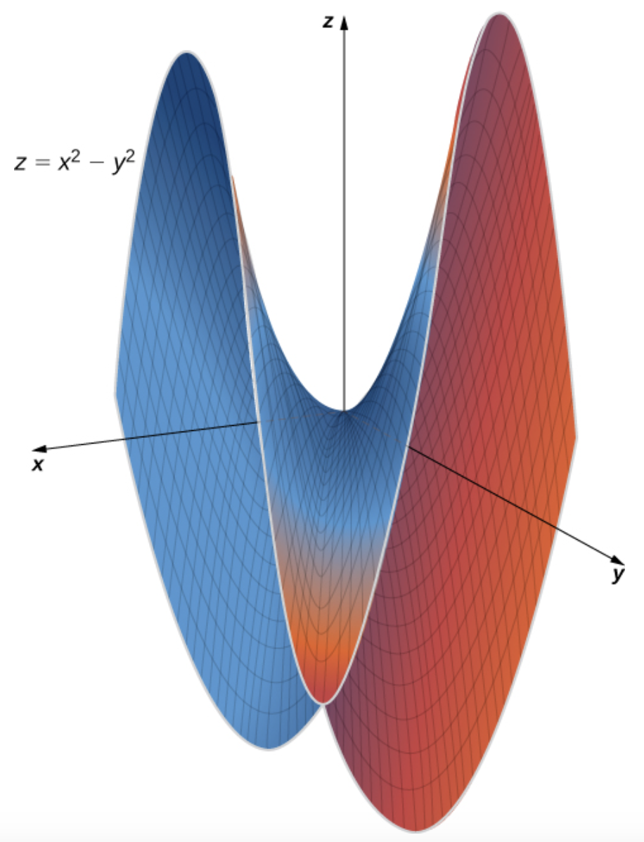
A saddle surface with the origin as the saddle point.
The 3D graph of \(z=y^2-x^2\) is shown with the saddle point at the origin. One cross-section curves upward like a valley, while the perpendicular cross-section curves downward like a ridge. The surface is colored blue on one side and red on the other, making the opposing curvatures visible.
Figure 5.5.2. A saddle point at the origin of the function \(f(x,y) = y^2 - x^2\text{.}\) Note that along the \(x\)-axis (\(y = 0\)), the function has a global maximum at \(x = 0\text{,}\) while along the \(y\)-axis (\(x = 0\)), the function has a global minimum at \(y = 0\text{.}\) This combination of maximum in one direction and minimum in another is characteristic of saddle points. Figure 4.48 from Edwin β€œJed” Herman and Gilbert Strang, Calculus Volume 3, OpenStax, Β© 2018 Rice University, licensed under CC BY-NC-SA 4.0; source: OpenStax Figure 4.48.
The second derivative test provides a method for determining whether a local extremum occurs at a critical point of a function. The test is more complicated for two-variable functions than the second derivative test for functions of a single variable, given that there are four second derivatives rather than just one derivative.

Remark 5.5.4.

From our current perspective, the second derivative test is quite mysterious. It seems unclear why the discriminant \(D\) is able to detect local extrema. We will later see in ActivityΒ 5.5.12, using our knowledge of linear algebra from UnitΒ 5, in particular the theory of eigenvalues, why the second derivative test detects local extrema, and also determine an analogue of the second derivative test for functions of more than two variables.

Activity 5.5.1.

Use the second derivative test to determine if the critical point \((1,-2)\) of \(f(x,y) = x^2 + y^2 - 2x + 4y\) found earlier is a local maximum, a local minimum, or a saddle point.
Solution.
We apply the second derivative test. We compute the second-order partial derivatives of \(f\text{.}\) We calculate that
\begin{equation*} f_{xx}(x,y) = 2 \quad f_{yy} = 2 \quad\text{and} \quad f_{xy}(x,y) = 0\text{.} \end{equation*}
So the discriminant is the constant function
\begin{equation*} D = f_{xx} f_{yy} - f_{xy}^2 = (2)(2) - (0)^2 = 4\text{.} \end{equation*}
Since the discriminant is positive, by the second derivative test, the critical point \((1,-2)\) is a local minimum.

Activity 5.5.2.

Use the second derivative test to analyze the critical point \((0,0)\) of \(f(x,y) = x^2 - y^2\) found earlier.
Solution.
We need to compute the second-order partial derivatives:
\begin{equation*} f_{xx} = 2 \quad f_{yy} = -2 \quad \text{and} \quad f_{xy} = 0\text{.} \end{equation*}
So the discriminant is also the constant function
\begin{equation*} D = f_{xx} f_{yy} - f_{xy}^2 = (2)(-2) - (0)^2 = -4\text{.} \end{equation*}
Since the discriminant is negative, the second derivative test tells us that \((0,0)\) is a saddle point of \(f\text{.}\)

Activity 5.5.3.

Find all local maxima, local minima, and saddle points for the function
\begin{equation*} f(x,y) = x^2 + xy + y^2 - 6x + 6\text{.} \end{equation*}
Solution.
We begin by finding the critical points of \(f\text{.}\) We calculate that
\begin{equation*} f_x(x,y)=2x+y-6 \qquad\text{and}\qquad f_y(x,y)=x+2y.\text{.} \end{equation*}
So the critical points satisfy
\begin{equation*} 2x+y-6=0 \qquad\text{and}\qquad x+2y=0. \end{equation*}
The second equation gives \(x=-2y\text{.}\) Substituting into the first equation gives
\begin{equation*} 2(-2y)+y-6=0, \end{equation*}
so \(-3y=6\text{,}\) and therefore \(y=-2\text{.}\) Thus \(x=4\text{,}\) and the only critical point is \((4,-2)\text{.}\)
To classify this critical point, we apply the second derivative test. We calculate that
\begin{equation*} f_{xx}(x,y)=2,\qquad f_{yy}(x,y)=2,\qquad f_{xy}(x,y)=1.\text{.} \end{equation*}
So the discriminant is the constant
\begin{equation*} D = f_{xx} f_{yy} - f_{xy}^2 = (2)(2) - (1)^2 = 3\text{.} \end{equation*}
Since \(D>0\) and \(f_{xx}>0\text{,}\) the critical point \((4,-2)\) is a local minimum.
In the previous examples, the discriminant of the functions were constant because \(f\) was a quadratic function. Let us consider an example where the discriminant is non-constant.

Activity 5.5.4.

Find all local maxima, local minima, and saddle points for the function \(f(x,y) = x^3 + y^2 + 2xy - 4x - 3y + 5\text{.}\)
Solution.
We begin by finding the critical point. We calculate that
\begin{equation*} f_x(x,y) = 3x^2 + 2y - 4 \quad\text{and}\quad f_y(x,y) = 2y + 2x - 3\text{.} \end{equation*}
Setting both equal to zero gives the pair of equations
\begin{equation*} 3x^2 + 2y - 4 = 0 \quad\text{and}\quad 2y + 2x - 3 = 0\text{.} \end{equation*}
We solve the second equation for \(y\text{,}\) i.e., that \(y = 3/2 - x\text{,}\) and then substitute this into the first equation, which leads to the equation
\begin{equation*} 3x^2 + 2(3/2 - x) - 4 = 0\text{,} \end{equation*}
which simplifies to the quadratic equation
\begin{equation*} 3x^2 - 2x - 1 = 0\text{.} \end{equation*}
The quadratic equation tells us that the roots of this equation are given by the formula
\begin{equation*} x = \frac{-(-2) \pm \sqrt{(-2)^2 - 4 (3)(-1)}}{2(3)} = 1/3 \pm \frac{\sqrt{16}}{6} = 1/3 \pm 2/3\text{.} \end{equation*}
So \(x = 1\) or \(x = -1/3\text{.}\) For each such \(x\text{,}\) setting \(y = 3/2 - x\) gives us a critical point for \(f\text{,}\) so \(f\) has two critical points, i.e., \((1,1/2)\) and \((-1/3,11/6)\text{.}\)
To apply the second derivative test to each critical point, we calculate the discriminant of \(f\text{.}\) We find that
\begin{equation*} f_{xx} = 6x \quad f_{yy} = 2 \quad \text{and}\quad f_{xy} = 2\text{.} \end{equation*}
So the discriminant is the function
\begin{equation*} D(x,y) = f_{xx}(x,y) f_{yy}(x,y) - f_{xy}(x,y)^2 = (6x)(2) - (2)^2 = 12x - 4\text{.} \end{equation*}
So
\begin{equation*} D(1,1/2) = 12(1) - 4 = 8 \quad\text{and}\quad D(-1/3,11/6) = 12(-1/3) - 4 = -8\text{.} \end{equation*}
Since \(D(1,1/2)\) is positive, and \(f_{xx}(1,1/2) = 6\) is positive, the critical point \((1,1/2)\) is a local minimum of the function \(f\text{.}\) Since \(D(-1/3,11/6)\) is negative, this tells us that \((-1/3,11/6)\) is a saddle point of the function \(f\text{.}\)

Remark 5.5.5.

The following activity explains why we only look at \(f_{xx}\) in the first two cases of the second derivative test.

Activity 5.5.5.

True or False: If \(D > 0\text{,}\) then \(f_{xx}\) and \(f_{yy}\) have the same sign.
Solution.
True. If \(D = f_{xx}f_{yy} - (f_{xy})^2 > 0\text{,}\) then \(f_{xx}f_{yy} > (f_{xy})^2 \geq 0\text{,}\) so \(f_{xx} f_{yy} > 0\text{.}\) Since \(f_{xx} f_{yy}\) is positive, this implies either both \(f_{xx}\) and \(f_{yy}\) are positive, or both \(f_{xx}\) and \(f_{yy}\) are negative. So \(f_{xx}\) and \(f_{yy}\) always have the same sign when the discriminant is positive.

Subsection Saddle points

Note 5.5.6.

A common way to detect a saddle point is to find two directions through the point such that the function increases in one direction and decreases in another. This is not a complete definition of every possible saddle point; it is a useful test in many examples.
For example, the function
\begin{equation*} f(x,y)=x^2-y^2 \end{equation*}
has a saddle point at \((0,0)\text{.}\) Along the line \(y=0\text{,}\)
\begin{equation*} f(x,0)=x^2, \end{equation*}
which has a local minimum at \(x=0\text{.}\) Along the line \(x=0\text{,}\)
\begin{equation*} f(0,y)=-y^2, \end{equation*}
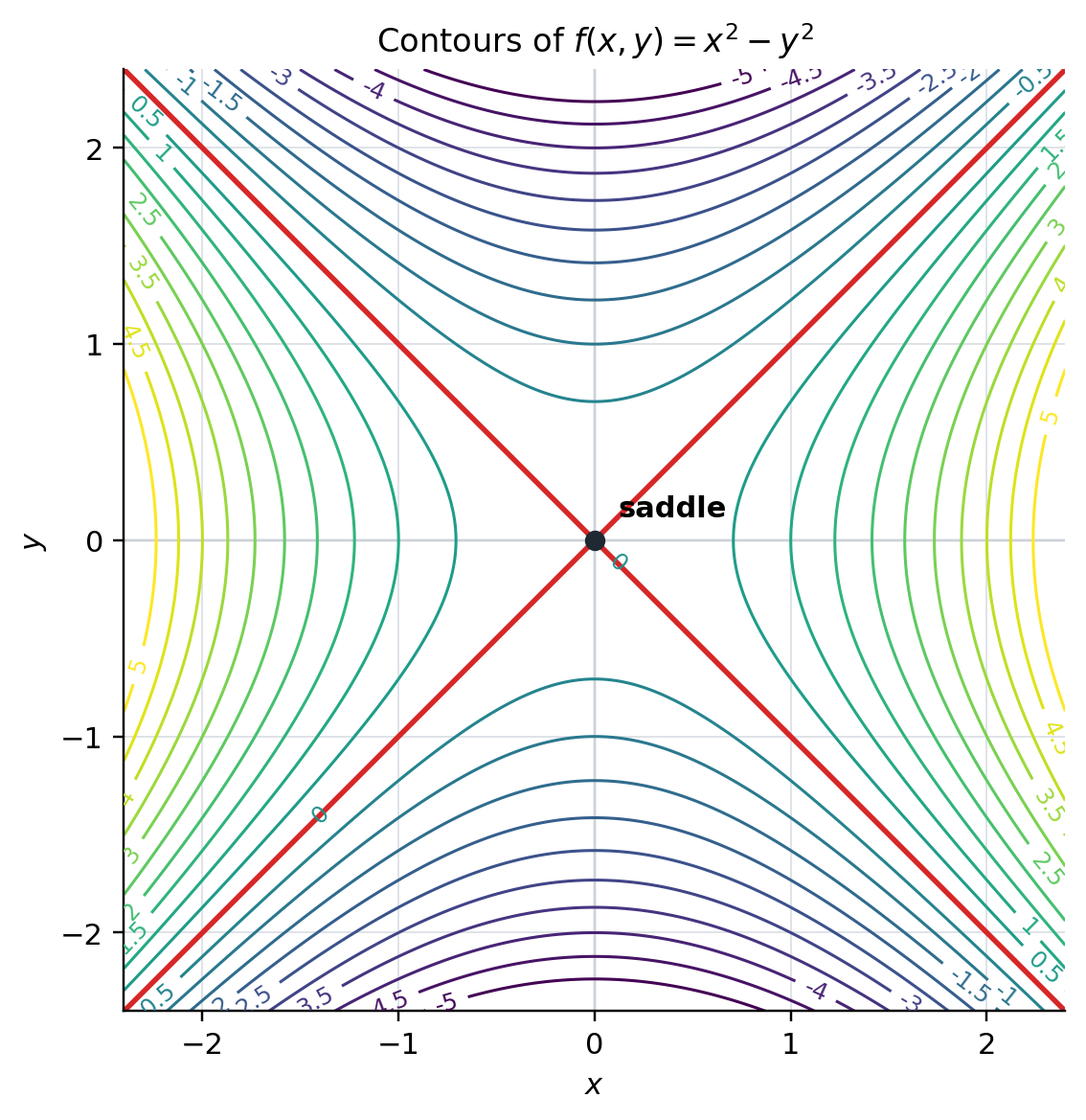
which has a local maximum at \(y=0\text{.}\) The contour plot below shows the same behavior.
In this example, the surface increases in one coordinate direction and decreases in the other. This is the behavior suggested by the saddle shape.
Contour plot of x squared minus y squared with a saddle point at the origin.
The contour plot shows level curves of \(f(x,y)=x^2-y^2\text{.}\) The zero contour consists of two diagonal lines crossing at the origin. Positive and negative contour values alternate across the four regions, indicating a saddle point at \((0,0)\text{.}\)
Figure 5.5.7. A contour plot of \(f(x,y) = x^2 - y^2\text{.}\) Adapted from: Stanford’s MATH 51 textbook.

Remark 5.5.8.

More formally, if the lines are given in parametric form by
\begin{equation*} \{\mathbf{a}+t\mathbf{d}_1\} \qquad\text{and}\qquad \{\mathbf{a}+t\mathbf{d}_2\}, \end{equation*}
then the one-variable restrictions
\begin{equation*} g(t)=f(\mathbf{a}+t\mathbf{d}_1) \qquad\text{and}\qquad h(t)=f(\mathbf{a}+t\mathbf{d}_2) \end{equation*}
can show opposite local behavior at \(t=0\text{.}\) In the example above, this verifies that nearby points occur on both sides of \(f(\mathbf{a})\text{.}\)
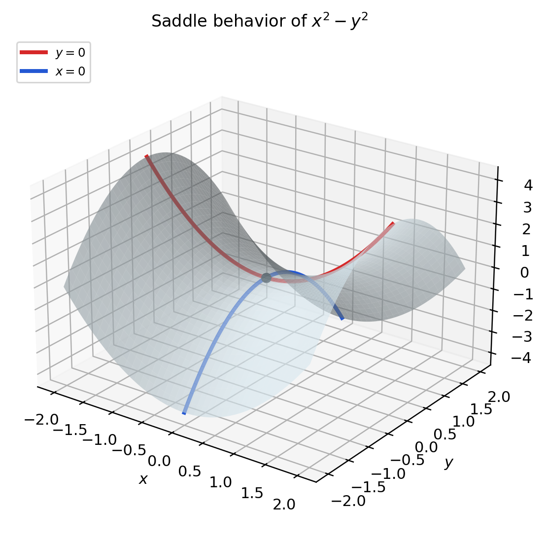
Saddle surface showing an upward x-axis slice and a downward y-axis slice.
A translucent saddle surface for \(z=x^2-y^2\) is shown. The red curve along \(y=0\) opens upward and has a local minimum at the origin, while the blue curve along \(x=0\) opens downward and has a local maximum at the origin.
Figure 5.5.9. At a saddle point for \(f(x,y)=x^2-y^2\text{,}\) there is a local minimum along \(y=0\) and a local maximum along \(x=0\text{.}\) Adapted from: Stanford’s MATH 51 textbook.

Activity 5.5.6.

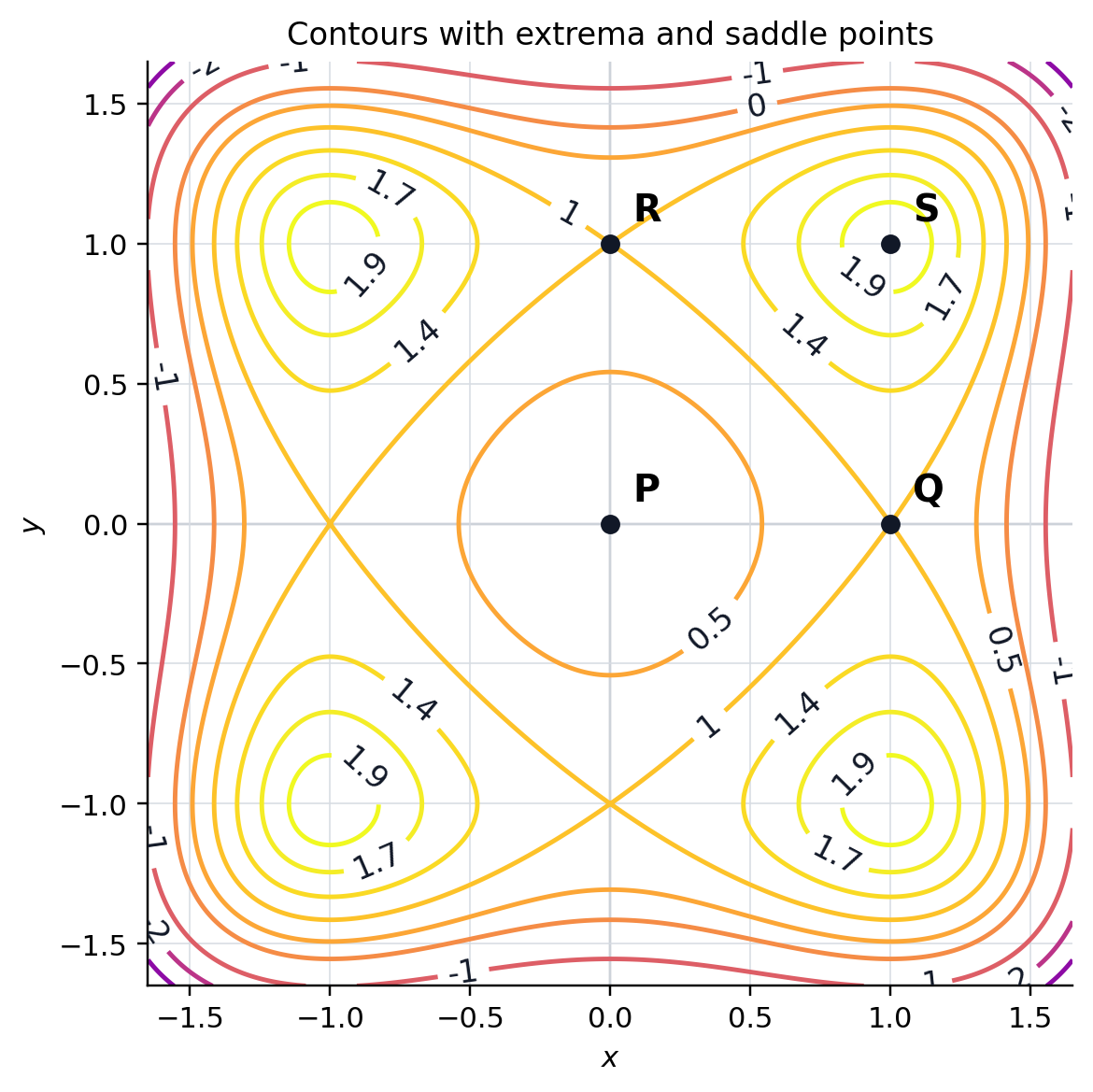
For each point in the figure below, indicate whether it is a local maximum, a local minimum, or a saddle point.
Contour plot with labeled local extrema and saddle points.
The contour plot shows level curves of the illustrative function \(g(x,y)=2-(x^2-1)^2-(y^2-1)^2\text{.}\) Point \(P\) is at the center of nested low-value contours, point \(S\) is at the center of nested high-value contours, and points \(Q\) and \(R\) are placed where the contour pattern changes like a saddle.
Figure 5.5.10. A contour plot with a variety of types of critical points. Adapted from: Stanford’s MATH 51 textbook.
Solution.
If we look at the collection of nested ovals centered on \(S\text{,}\) and inspect the numerical values labeling the level sets, we see those numbers are strictly increasing. These ovals seem to be honing in on a point \(S\) that is a local maximum. Likewise, the collection of nested ovals near \(P\) have function values going in a decreasing direction, suggesting \(P\) is a local minimum. We also see saddle points at \(R\) and \(Q\text{.}\) As we move away from \(R\) in the north-east direction, the function value increases, whereas moving away in the south-east direction causes the function value to decrease. Near saddle points, the contour plot forms an "X" shape dividing the space into \(4\) regions. Function values increase in one pair of opposite regions and decrease in the other pair. Near local extrema, level sets form oval shapes resembling ellipses.

Subsection The second derivative test

In this subsection, we now obtain a form of the second derivative test for scalar-valued functions with more than two variables.

Subsubsection Quadratic approximation and quadratic forms

Recall that if a single-variable function \(f\) has \(n\) derivatives at \(x = a\text{,}\) then the \(n\)th Taylor polynomial for \(f\) at \(a\) is the function
\begin{align*} p_n(x) \amp = f(a) + f'(a)(x - a) + \frac{f''(a)}{2!}(x - a)^2 + \cdots + \frac{f^{(n)}(a)}{n!}(x - a)^n\\ \amp = \sum_{k=0}^n \frac{f^{(k)}(a)}{k!}(x - a)^k\text{.} \end{align*}
In particular, for \(n = 1\) we obtain the linear approximation
\begin{equation*} p_1(x) = f(a) + f'(a) (x - a) \end{equation*}
of \(f\text{,}\) and for \(n = 2\) we obtain the quadratic approximation
\begin{equation*} p_2(x) = f(a) + f'(a) (x - a) + f''(a) \frac{(x-a)^2}{2}\text{.} \end{equation*}
The Taylor polynomial \(p_n(x)\) approximates the function \(f(x)\) near \(x = a\text{,}\) with the approximation improving as \(n\) increases.
Activity 5.5.7.
Consider the function \(f(x) = \sqrt[3]{x}\text{.}\)
(a) Find the first and second Taylor polynomials for \(f\) at \(x = 8\text{.}\)
Solution.
For \(f(x) = \sqrt[3]{x}\text{,}\) the values of the function and its first two derivatives at \(x = 8\) are as follows:
\begin{align*} f(x) \amp = \sqrt[3]{x} \amp f(8) \amp = 2\\ f'(x) \amp = \frac{1}{3x^{2/3}} \amp f'(8) \amp = \frac{1}{12}\\ f''(x) \amp = \frac{-2}{9x^{5/3}} \amp f''(8) \amp = -\frac{1}{144} \end{align*}
Thus, the first and second Taylor polynomials at \(x = 8\) are given by:
\begin{align*} p_1(x) \amp = f(8) + f'(8)(x - 8)\\ \amp = 2 + \frac{1}{12}(x - 8)\\ p_2(x) \amp = f(8) + f'(8)(x - 8) + \frac{f''(8)}{2!}(x - 8)^2\\ \amp = 2 + \frac{1}{12}(x - 8) - \frac{1}{288}(x - 8)^2 \end{align*}
Activity 5.5.8.
(b) Use these two polynomials to estimate \(\sqrt[3]{11}\text{.}\)
Solution.
Using the first Taylor polynomial at \(x = 8\text{,}\) we can estimate:
\begin{align*} \sqrt[3]{11} \approx p_1(11) \amp = 2 + \frac{1}{12}(11 - 8)\\ \amp = 2.25 \end{align*}
Using the second Taylor polynomial at \(x = 8\text{,}\) we obtain:
\begin{align*} \sqrt[3]{11} \approx p_2(11) \amp = 2 + \frac{1}{12}(11 - 8) - \frac{1}{288}(11 - 8)^2\\ \amp = 2 + \frac{1}{4} - \frac{1}{32}\\ \amp = 2.21875 \end{align*}
If \(a\) is a critical point of \(f\text{,}\) then the quadratic approximation of \(f\) is given by the expression
\begin{equation*} f(a) + f''(a) \frac{(x-a)^2}{2} \end{equation*}
If \(f''(a) \gt 0\text{,}\) then the quadratic approximation of \(f\) is an upward pointing parabola with a vertex at \((a,f(a))\text{.}\) This approximation has a minimum at this vertex, explaining \(a\) is a local minimum of the function \(f\) (since \(f\) is closely approximated by its quadratic approximation). Similarly, if \(f''(a) \lt 0\text{,}\) then the quadratic approximation is a downward pointing parabola with a maximum at \((a,f(a))\text{,}\) explaining why \(a\) is a local maximum of the function \(f\text{.}\)
This explanation indicates how the second derivative test might work for a multi variable function. We obtain an analogue of the quadratic approximation of such a function. Then, if that quadratic approximation has a maximum or minumum at the critical point, then the actual function has a local minimum or maximum near that point. The quadratic approximation of the function \(f\) is defined in terms of the Hessian of \(f\) (recall DefinitionΒ 3.4.17).
Definition 5.5.11. Quadratic approximation.
The quadratic approximation \(Q(\mathbf{x})\) of a scalar-valued function \(f\) near a point \(\mathbf{a}\) is the function defined by
\begin{equation*} Q(\mathbf{x}) = f(\mathbf{a}) + \nabla f(\mathbf{a})\cdot(\mathbf{x}-\mathbf{a}) + \frac12(\mathbf{x}-\mathbf{a})^T H_f(\mathbf{a})(\mathbf{x}-\mathbf{a}).\text{.} \end{equation*}
Remark 5.5.12.
The quadratic approximation of a function \(f\) refines the linear approximation via the gradient that we previously encountered. In particular, if the second derivatives of \(f\) are continuous, then
\begin{equation*} \lim_{\mathbf{x} \to \mathbf{a}} \frac{f(\mathbf{x}) - Q(\mathbf{x})}{\| \mathbf{x} - \mathbf{a} \|^2} = 0\text{.} \end{equation*}
If \(\mathbf{x}\) is close to \(\mathbf{a}\text{,}\) then \(\| \mathbf{x} - \mathbf{a} \|^2\) is much smaller than \(\| \mathbf{x} - \mathbf{a} \|\text{,}\) so that the quadratic approximation \(Q(\mathbf{x})\) to \(f\) is in general a much better approximation thatn the linear approximation \(L(\mathbf{x})\text{.}\)
Activity 5.5.9.
Compute the gradient and the Hessian of the function \(f(x, y) = \ln(xy - 1)\) at the point \((x, y) = (1, 2)\text{,}\) use these values to determine the quadratic approximation to \(f\) at the point \((1,2)\text{,}\) and then use the quadratic approximation to estimate the value of \(f\) at \((1.2, 1.8)\text{.}\)
Solution.
We calculate that
\begin{equation*} f_x = \frac{y}{xy - 1} \quad\text{and}\quad f_y = \frac{x}{xy - 1}\text{.} \end{equation*}
So \((\nabla f)(1,2) = (2,1)\text{.}\) Next, we compute that
\begin{align*} f_{xx} \amp = \frac{-y^2}{(xy - 1)^2} \amp f_{yy} \amp = \frac{-x^2}{(xy - 1)^2} \amp f_{xy} \amp = f_{yx} = \frac{-1}{(xy - 1)^2}\text{.} \end{align*}
Evaluating at \((1, 2)\text{,}\) we find that
\begin{equation*} H_f(1, 2) = \begin{bmatrix} \frac{-4}{1} \amp \frac{-1}{1} \\ \frac{-1}{1} \amp \frac{-1}{1} \end{bmatrix} = \begin{bmatrix} -4 \amp -1 \\ -1 \amp -1 \end{bmatrix}\text{.} \end{equation*}
Since
\begin{equation*} f(1,2) = \ln(1) = 0\text{,} \end{equation*}
using the Hessian and gradient, we find that the quadratic approximation of \(f\) near \((1,2)\) is given by
\begin{align*} Q(x,y) \amp = (2,1) \cdot ( x - 1, y - 2 ) + \frac{1}{2} \begin{bmatrix} x - 1 \amp y - 2 \end{bmatrix} \begin{bmatrix} -4 \amp -1 \\ -1 \amp -1 \end{bmatrix} \begin{bmatrix} x - 1 \\ y - 2 \end{bmatrix}\\ \amp = 2(x - 1) + (y-2) - 2 (x - 1)^2 - (x-1)(y-2) - (1/2) (y-2)^2\text{.} \end{align*}
So
\begin{align*} Q(1.2,1.8) \amp = 2(0.2) + (-0.2) - 2 (0.2)^2 - (0.2)(-0.2) - (1/2) (-0.2)^2\\ \amp = 0.4 - 0.2 - 0.08 + 0.04 - 0.02\\ \amp = 0.14\text{.} \end{align*}
Up to four decimals, the best approximation of \(f(1.2,1.8)\) is \(0.1484\text{,}\) so the quadratic approximation is quite accurate. For comparison, the linear comparison \(L\) at \((1,2)\) is given by
\begin{equation*} L(x,y) =2(0.2) + (-0.2) = 0.2\text{,} \end{equation*}
which is far less accurate.
Activity 5.5.10.
Let \(f(x, y) = \cos(x/y)\text{.}\) Use the gradient and Hessian to obtain a quadratic approximation of the function \(f(x, y)\) near \(\mathbf{a} = (0, 1)\text{.}\)
Solution.
We calculate that
\begin{equation*} \nabla f(x,y) = \left( - \frac{\sin(x/y)}{y}, \frac{x \sin(x/y)}{y^2} \right) \end{equation*}
In particular, \(\nabla f(0,1) = (0,0)\text{.}\) Next, we calculate that
\begin{align*} \amp f_{xx} = -\frac{1}{y^2}\cos\left(\frac{x}{y}\right), \quad f_{yy} = \frac{x}{y^4}\left(2y\sin\left(\frac{x}{y}\right) + x\cos\left(\frac{x}{y}\right)\right)\\ \amp f_{xy} = f_{yx} = \frac{1}{y^3}\left(y\sin\left(\frac{x}{y}\right) + x\cos\left(\frac{x}{y}\right)\right) \end{align*}
So
\begin{equation*} H_f(0,1) = \begin{bmatrix} -1 \amp 0 \\ 0 \amp 0 \end{bmatrix} \end{equation*}
Since \(f(0,1) = \cos(0) = 1\text{,}\) the quadratic approximation of \(f\) at \((0,1)\) is thus given by
\begin{equation*} Q(x,y) = 1 - x^2/2\text{.} \end{equation*}
If \(\mathbf{a}\) is a critical point of a function \(f\text{,}\) then the quadratic approximation of the function \(f\) takes the form
\begin{equation*} Q(\mathbf{x}) = f(\mathbf{a}) + \frac{1}{2} (\mathbf{x} - \mathbf{a})^T H_f(\mathbf{a}) (\mathbf{x} - \mathbf{a})\text{,} \end{equation*}
and so it suffices to understand the quadratic form associated with the Hessian matrix.

Subsubsection The second derivative test

Why is this true?.
At a critical point, the first-order term in the Taylor approximation is zero. For small \(\mathbf{h}\text{,}\)
\begin{equation*} f(\mathbf{a}+\mathbf{h})-f(\mathbf{a}) = \frac12\mathbf{h}^T H_f(\mathbf{a})\mathbf{h} + \text{terms smaller than }\|\mathbf{h}\|^2. \end{equation*}
If \(H_f(\mathbf{a})\) is positive definite, then the quadratic term is positive for every nonzero sufficiently small \(\mathbf{h}\text{,}\) so \(f(\mathbf{a}+\mathbf{h})>f(\mathbf{a})\) for all sufficiently small nonzero \(\mathbf{h}\text{.}\) This gives a local minimum. The negative definite case gives a local maximum. If the Hessian is indefinite, there are directions in which the quadratic term is positive and directions in which it is negative, so nearby points occur on both sides of \(f(\mathbf{a})\text{.}\) This gives a saddle point.
Activity 5.5.11. Predicting from Hessian eigenvalues.
Suppose \(\mathbf{a}\) is a critical point of a scalar-valued function \(f\text{.}\) For each list of eigenvalues of \(H_f(\mathbf{a})\text{,}\) classify the critical point as a local minimum, local maximum, saddle point, or inconclusive.
  1. \(\displaystyle 3,5\)
  2. \(\displaystyle -2,-7\)
  3. \(\displaystyle 4,-1\)
  4. \(\displaystyle 0,2\)
Tags. [U5-LO5 | C+R | Core]
Solution.
If the eigenvalues are \(3,5\text{,}\) then the Hessian is positive definite, so the critical point is a local minimum.
If the eigenvalues are \(-2,-7\text{,}\) then the Hessian is negative definite, so the critical point is a local maximum.
If the eigenvalues are \(4,-1\text{,}\) then the Hessian is indefinite, so the critical point is a saddle point.
If the eigenvalues are \(0,2\text{,}\) the test is inconclusive. The zero eigenvalue means the second-order approximation has a flat direction, so the second derivative test alone does not decide the local behavior.
Activity 5.5.12.
Show that a matrix
\begin{equation*} A = \begin{bmatrix} a \amp b \\ b \amp d \end{bmatrix} \end{equation*}
is positive definite if and only if \(ad - b^2\) is positive and \(a > 0\text{,}\) negative definite if and only if \(ad - b^2\) is positive and \(a \lt 0\text{,}\) and indefinite if and only if \(ad - b^2\) is negative. It follows from this that the second derivative test in two variables is just a special case of the second derivative test above.
Solution.
If \(A\) has eigenvalues \(\lambda_1\) and \(\lambda_2\text{,}\) then \(ad - b^2 = \lambda_1 \lambda_2\) (the determinant of two similar matrices is the same). So if \(ad - b^2\) is positive, \(\lambda_1\) and \(\lambda_2\) are either both positive (and the matrix is positive definite) or both negative (and so the matrix is negative definite). Conversely, if \(ad - b^2\) is negative, \(\lambda_1\) and \(\lambda_2\) have opposite signs, so the matrix is indefinite.
If \(ad - b^2\) is positive, then \(ad\) is positive. If \(a\) and \(d\) are both positive, then the characteristic polynomial of this matrix is given by
\begin{equation*} (\lambda - a) (\lambda - d) - b^2 = \lambda^2 - (a + d) \lambda + (ad - b^2)\text{.} \end{equation*}
This is a quadratic equation with vertex at
\begin{equation*} \lambda = \frac{a + d}{2}\text{,} \end{equation*}
which is positive. There must exist a root of the equation to the right of the vertex, so the characteristic polynomial has a positive root (and thus both roots are positive). Conversely, if \(a\) and \(d\) are both negative, then the characteristic polynomial has a vertex to the left of the \(y\)-axis, and so has a negative root (and thus both roots are negative).
Activity 5.5.13.
Consider the function \(f(x,y,z) = x^2 + y^2 - xz\text{.}\) Find all critical points of \(f\) and determine the behavior of \(f\) near each critical point.
(a)
First find the critical points.
Solution.
We compute that \(\nabla f(x,y,z) = ( 2x - z, 2y, -x )\text{,}\) which vanishes only at \((0,0,0)\text{,}\) which is the only critical point.
(b)
Now classify each critical point.
Solution.
The Hessian is the constant matrix
\begin{equation*} H_f = \begin{bmatrix} 2 \amp 0 \amp -1 \\ 0 \amp 2 \amp 0 \\ -1 \amp 0 \amp 0 \end{bmatrix}\text{.} \end{equation*}
The associated quadratic form is
\begin{align*} \mathbf{h}^T H_f\mathbf{h} \amp = 2h_1^2+2h_2^2-2h_1h_3.\text{.} \end{align*}
This quadratic form takes both positive and negative values. For example,
\begin{equation*} \begin{bmatrix}0\\1\\0\end{bmatrix}^T H_f \begin{bmatrix}0\\1\\0\end{bmatrix} =2>0, \end{equation*}
but
\begin{equation*} \begin{bmatrix}1\\0\\3\end{bmatrix}^T H_f \begin{bmatrix}1\\0\\3\end{bmatrix} = 2-6=-4\lt 0. \end{equation*}
Thus \(H_f\) is indefinite. By the second derivative test, the critical point \((0,0,0)\) is a saddle point.
Activity 5.5.14.
Classify the critical points of the function \(f(x,y,z) = xy + yz + xz + xyz\) using the second derivative test.
Solution.
We compute that
\begin{equation*} \nabla f(x,y,z) = \begin{bmatrix} y + z + yz\\ x + z + xz\\ x + y + xy \end{bmatrix}\text{.} \end{equation*}
Notice that \(\nabla f(x,-1,z) = ( -1, x + z + xz, -1 )\) is non-vanishing, so that there are no critical points on the plane \(y = -1\text{.}\) Now suppose that \(\nabla f(x,y,z) = 0\) and \(y \neq -1\text{.}\) The third entry tells us that \(x = -y/(1 + y)\text{.}\) Substituting this into the second equation gives that \(-y/(1+y) + z - yz/(1+y) = 0\text{,}\) i.e., that \(z = y\text{.}\) Substituting this into the first equation gives that \(y^2 + 2y = 0\text{,}\) i.e., that \(y = 0\) or \(y = -2\text{.}\) Substituting back gives the two critical points of \(f\text{,}\) namely \((0,0,0)\) and \((-2,-2,-2)\text{.}\)
Next, we classify these critical points. We calculate that the Hessian of \(f\) is
\begin{equation*} H_f(x,y,z) = \begin{bmatrix} 0 \amp 1 + z \amp 1 + y \\ 1 + z \amp 0 \amp 1 + x \\ 1 + y \amp 1 + x \amp 0 \end{bmatrix}\text{.} \end{equation*}
In particular,
\begin{equation*} H_f(0,0,0) = \begin{bmatrix} 0 \amp 1 \amp 1 \\ 1 \amp 0 \amp 1 \\ 1 \amp 1 \amp 0 \end{bmatrix}\text{,} \end{equation*}
which has characteristic polynomial
\begin{align*} \det \begin{bmatrix} \lambda \amp -1 \amp -1 \\ -1 \amp \lambda \amp -1 \\ -1 \amp -1 \amp \lambda \end{bmatrix} \amp = \lambda( \lambda^2 - 1) - (-1) (-\lambda - 1) + (-1) (1 + \lambda)\\ \amp = \lambda^3 - 3\lambda - 2\\ \amp = (\lambda + 1)(\lambda^2 - \lambda - 2)\\ \amp = (\lambda + 1)^2( \lambda - 2 )\text{.} \end{align*}
So \(H_f(0,0,0)\) has eigenvalues \(-1\) and \(2\text{,}\) and so is indefinite, so that \(f\) has a saddle point at \((0,0,0)\text{.}\) We have
\begin{equation*} H_f(-2,-2,-2) = \begin{bmatrix} 0 \amp -1 \amp -1 \\ -1 \amp 0 \amp -1 \\ -1 \amp -1 \amp 0 \end{bmatrix}\text{,} \end{equation*}
which has characteristic polynomial
\begin{align*} \det \begin{bmatrix} \lambda \amp 1 \amp 1 \\ 1 \amp \lambda \amp 1 \\ 1 \amp 1 \amp \lambda \end{bmatrix} \amp = \lambda( \lambda^2 - 1) - (\lambda - 1) + (1 - \lambda)\\ \amp = \lambda^3 - 3 \lambda + 2\\ \amp = (\lambda - 1)(\lambda^2 + \lambda - 2)\\ \amp = (\lambda - 1)^2(\lambda + 2)\text{,} \end{align*}
so \(H_f(-2,-2,-2)\) has eigenvalues \(1\) and \(-2\text{,}\) and is thus an indefinite matrix. So \((-2,-2,-2)\) is also a saddle point of \(f\text{.}\)