Skip to main content
Contents Dark Mode Prev Up Next \(\newcommand{\N}{\mathbb{N}}
\newcommand{\Z}{\mathbb{Z}}
\newcommand{\Q}{\mathbb{Q}}
\newcommand{\R}{\mathbb{R}}
\newcommand{\dimens}{\operatorname{dim}}
\DeclareMathOperator{\row}{\operatorname{row}}
\DeclareMathOperator{\col}{\operatorname{col}}
\newcommand{\im}{\operatorname{im}}
\newcommand{\nulls}{\operatorname{null}}
\newcommand{\minor}{\operatorname{minor}}
\newcommand{\spans}{\operatorname{span}}
\newcommand{\nullity}{\operatorname{nullity}}
\newcommand{\kers}{\operatorname{ker}}
\newcommand{\proj}{\operatorname{proj}}
\newcommand{\diag}{\operatorname{diag}}
\newcommand{\Tr}{\operatorname{Tr}}
\newcommand{\rank}{\operatorname{rank}}
\newcommand{\lt}{<}
\newcommand{\gt}{>}
\newcommand{\amp}{&}
\definecolor{fillinmathshade}{gray}{0.9}
\newcommand{\fillinmath}[1]{\mathchoice{\colorbox{fillinmathshade}{$\displaystyle \phantom{\,#1\,}$}}{\colorbox{fillinmathshade}{$\textstyle \phantom{\,#1\,}$}}{\colorbox{fillinmathshade}{$\scriptstyle \phantom{\,#1\,}$}}{\colorbox{fillinmathshade}{$\scriptscriptstyle\phantom{\,#1\,}$}}}
\)
Section 4.3 Least squares as projection
Unit 2 2.2.24 asked whether a target vector
\(\mathbf{b}\) is reachable as
\(A\mathbf{x}\text{.}\) When
\(\mathbf{b}\notin\operatorname{col}(A)\text{,}\) no input reaches the target exactly. Least squares replaces the unreachable target by the closest reachable output. Recall the Unit 2 matrix and target
\begin{equation*}
A=
\begin{bmatrix}
1\amp 0\\
0\amp 1\\
1\amp 1
\end{bmatrix},
\qquad
\mathbf{b}=
\begin{bmatrix}
1\\
2\\
4
\end{bmatrix}.
\end{equation*}
For
\begin{equation*}
\mathbf{x}=
\begin{bmatrix}
x_1\\
x_2
\end{bmatrix},
\end{equation*}
we have
\begin{equation*}
A\mathbf{x}
=
\begin{bmatrix}
x_1\\
x_2\\
x_1+x_2
\end{bmatrix}.
\end{equation*}
Every reachable output therefore has third coordinate equal to the sum of its first two coordinates. The target \(\mathbf{b}\) is not reachable because \(4\neq 1+2\text{.}\)
Definition 4.3.1 . Least-squares solution, fitted vector, and residual.
Let \(A\) be an \(m\times n\) matrix and let \(\mathbf{b}\in\mathbb{R}^m\text{.}\) A least-squares solution is a vector \(\widehat{\mathbf{x}}\in\mathbb{R}^n\) that minimizes
\begin{equation*}
\|A\mathbf{x}-\mathbf{b}\|^2
\end{equation*}
over all \(\mathbf{x}\in\mathbb{R}^n\text{.}\) The vector
\begin{equation*}
\widehat{\mathbf{b}}=A\widehat{\mathbf{x}}
\end{equation*}
is the fitted vector. The vector
\begin{equation*}
\mathbf{r}
=
\mathbf{b}-\widehat{\mathbf{b}}
=
\mathbf{b}-A\widehat{\mathbf{x}}
\end{equation*}
is the residual.
The quantity
\begin{equation*}
\|A\mathbf{x}-\mathbf{b}\|^2
=
\sum_{i=1}^m
\bigl((A\mathbf{x})_i-b_i\bigr)^2
\end{equation*}
is the sum of the squares of the coordinate errors. This explains the name least squares. Minimizing the norm or its square gives the same minimizers. If \(\mathbf{b}\in\operatorname{col}(A)\text{,}\) the minimum error is \(0\text{,}\) and least squares agrees with solving \(A\mathbf{x}=\mathbf{b}\) exactly. If the target is not reachable, the fitted vector \(\widehat{\mathbf{b}}\) is the closest reachable output.
\begin{equation*}
\widehat{\mathbf{b}}=A\widehat{\mathbf{x}}.
\end{equation*}
The residual is
\begin{equation*}
\mathbf{r}
=
\mathbf{b}-\widehat{\mathbf{b}}.
\end{equation*}
The projection theorem guarantees a closest vector \(\widehat{\mathbf{b}}\in\operatorname{col}(A)\text{.}\) Since \(\widehat{\mathbf{b}}\) lies in the column space, at least one coefficient vector \(\widehat{\mathbf{x}}\) satisfies
\begin{equation*}
A\widehat{\mathbf{x}}=\widehat{\mathbf{b}}.
\end{equation*}
Fact 4.3.2 . \(A^T\) checks column orthogonality.
Write
\begin{equation*}
A=
\begin{bmatrix}
\mathbf{a}_1\amp\cdots\amp\mathbf{a}_n
\end{bmatrix}.
\end{equation*}
For any vector \(\mathbf{r}\in\mathbb{R}^m\text{,}\)
\begin{equation*}
A^T\mathbf{r}
=
\begin{bmatrix}
\mathbf{a}_1^T\mathbf{r}\\
\vdots\\
\mathbf{a}_n^T\mathbf{r}
\end{bmatrix}.
\end{equation*}
Therefore
\begin{equation*}
A^T\mathbf{r}=\mathbf{0}
\end{equation*}
exactly when \(\mathbf{r}\) is orthogonal to every column of \(A\text{.}\) Equivalently,
\begin{equation*}
\operatorname{col}(A)^\perp
=
\operatorname{null}(A^T).
\end{equation*}
Every fitted vector \(A\mathbf{x}\) lies in \(\operatorname{col}(A)\text{.}\) Therefore the least-squares fitted vector is
\begin{equation*}
\widehat{\mathbf{b}}
=
A\widehat{\mathbf{x}}
=
\operatorname{proj}_{\operatorname{col}(A)}(\mathbf{b}).
\end{equation*}
Its residual
\begin{equation*}
\mathbf{r}
=
\mathbf{b}-A\widehat{\mathbf{x}}
\end{equation*}
is orthogonal to \(\operatorname{col}(A)\text{.}\)
Theorem 4.3.3 . Least squares and the normal equations.
A vector \(\widehat{\mathbf{x}}\) is a least-squares solution exactly when the residual
\begin{equation*}
\mathbf{r}
=
\mathbf{b}-A\widehat{\mathbf{x}}
\end{equation*}
is orthogonal to \(\operatorname{col}(A)\text{.}\) Equivalently,
\begin{equation*}
A^T
\bigl(
\mathbf{b}-A\widehat{\mathbf{x}}
\bigr)
=
\mathbf{0}.
\end{equation*}
Thus the least-squares solutions are exactly the solutions of the normal equations
\begin{equation*}
A^TA\widehat{\mathbf{x}}
=
A^T\mathbf{b}.
\end{equation*}
Why is this true?.
Every candidate fitted vector
\(A\mathbf{x}\) lies in
\(\operatorname{col}(A)\text{.}\) By the
projection theorem 4.2.8 ,
\(A\widehat{\mathbf{x}}\) is closest to
\(\mathbf{b}\) exactly when
\begin{equation*}
\mathbf{b}-A\widehat{\mathbf{x}}
\in
\operatorname{col}(A)^\perp.
\end{equation*}
By the fact above, this is equivalent to
\begin{equation*}
A^T
\bigl(
\mathbf{b}-A\widehat{\mathbf{x}}
\bigr)
=
\mathbf{0}.
\end{equation*}
Expanding and rearranging gives
\begin{equation*}
A^T\mathbf{b}
-
A^TA\widehat{\mathbf{x}}
=
\mathbf{0},
\end{equation*}
or
\begin{equation*}
A^TA\widehat{\mathbf{x}}
=
A^T\mathbf{b}.
\end{equation*}
The fitted vector \(\widehat{\mathbf{b}}\) is unique because orthogonal projection onto a subspace is unique. The coefficient vector \(\widehat{\mathbf{x}}\) need not be unique. If \(\mathbf{z}\in\operatorname{null}(A)\text{,}\) then
\begin{equation*}
A
\bigl(
\widehat{\mathbf{x}}+\mathbf{z}
\bigr)
=
A\widehat{\mathbf{x}}.
\end{equation*}
When the columns of \(A\) are linearly independent, \(\operatorname{null}(A)=\{\mathbf{0}\}\text{,}\) so the least-squares coefficient vector is unique.
Activity 4.3.4 . Independent columns and \(A^TA\) (U2-LO5).
Let \(A\) be an \(m\times n\) matrix. Use the identity
\begin{equation*}
\mathbf{x}^TA^TA\mathbf{x}
=
\|A\mathbf{x}\|^2
\end{equation*}
to explain why \(A^TA\) is invertible exactly when the columns of \(A\) are linearly independent.
Suppose
\begin{equation*}
A^TA\mathbf{x}=\mathbf{0}.
\end{equation*}
What does the displayed identity say about \(\|A\mathbf{x}\|^2\text{?}\)
If the columns of
\(A\) are linearly independent, what must
\(\mathbf{x}\) be?
Conversely, suppose \(A^TA\) is invertible and
\begin{equation*}
A\mathbf{x}=\mathbf{0}.
\end{equation*}
What equation results after multiplying by \(A^T\text{?}\)
Explain why the two conditions are equivalent.
Solution .
If
\begin{equation*}
A^TA\mathbf{x}=\mathbf{0},
\end{equation*}
then
\begin{equation*}
0
=
\mathbf{x}^TA^TA\mathbf{x}
=
\|A\mathbf{x}\|^2.
\end{equation*}
Therefore \(A\mathbf{x}=\mathbf{0}\text{.}\) If the columns of \(A\) are linearly independent, then
\begin{equation*}
\operatorname{null}(A)=\{\mathbf{0}\},
\end{equation*}
so \(\mathbf{x}=\mathbf{0}\text{.}\) Thus \(\operatorname{null}(A^TA)=\{\mathbf{0}\}\text{,}\) and the square matrix \(A^TA\) is invertible.
Conversely, suppose \(A^TA\) is invertible and
\begin{equation*}
A\mathbf{x}=\mathbf{0}.
\end{equation*}
Multiplying by \(A^T\) gives
\begin{equation*}
A^TA\mathbf{x}=\mathbf{0}.
\end{equation*}
Since \(A^TA\) is invertible, \(\mathbf{x}=\mathbf{0}\text{.}\) Therefore
\begin{equation*}
\operatorname{null}(A)=\{\mathbf{0}\},
\end{equation*}
so the columns of \(A\) are linearly independent.
Activity 4.3.5 . Unit 2 target revisited (U4-LO4, U4-LO5).
Let
\begin{equation*}
A=
\begin{bmatrix}
1\amp 0\\
0\amp 1\\
1\amp 1
\end{bmatrix},
\qquad
\mathbf{b}=
\begin{bmatrix}
1\\
2\\
4
\end{bmatrix}.
\end{equation*}
Recall why
\(A\mathbf{x}=\mathbf{b}\) has no exact solution.
Form
\(A^TA\) and
\(A^T\mathbf{b}\text{.}\)
Solve the normal equations for
\(\widehat{\mathbf{x}}\text{.}\)
Compute the fitted vector
\begin{equation*}
\widehat{\mathbf{b}}
=
A\widehat{\mathbf{x}}
\end{equation*}
and the residual
\begin{equation*}
\mathbf{r}
=
\mathbf{b}-\widehat{\mathbf{b}}.
\end{equation*}
Check that
\begin{equation*}
A^T\mathbf{r}=\mathbf{0}.
\end{equation*}
Compute
\(\|\mathbf{r}\|^2\text{.}\)
Which vector is the closest reachable output:
\(\widehat{\mathbf{x}}\) or
\(\widehat{\mathbf{b}}\text{?}\)
The residual is not zero. Explain why this does not mean least squares failed.
Solution .
For
\begin{equation*}
\mathbf{x}
=
\begin{bmatrix}
x_1\\
x_2
\end{bmatrix},
\end{equation*}
we have
\begin{equation*}
A\mathbf{x}
=
\begin{bmatrix}
x_1\\
x_2\\
x_1+x_2
\end{bmatrix}.
\end{equation*}
The first two coordinates of \(A\mathbf{x}=\mathbf{b}\) would force \(x_1=1\) and \(x_2=2\text{,}\) but then the third coordinate would be \(3\text{,}\) not \(4\text{.}\) Thus the target is not reachable exactly.
The normal equations use
\begin{equation*}
A^TA
=
\begin{bmatrix}
2\amp 1\\
1\amp 2
\end{bmatrix},
\qquad
A^T\mathbf{b}
=
\begin{bmatrix}
5\\
6
\end{bmatrix}.
\end{equation*}
Solving
\begin{equation*}
\begin{bmatrix}
2\amp 1\\
1\amp 2
\end{bmatrix}
\widehat{\mathbf{x}}
=
\begin{bmatrix}
5\\
6
\end{bmatrix}
\end{equation*}
gives
\begin{equation*}
\widehat{\mathbf{x}}
=
\begin{bmatrix}
4/3\\
7/3
\end{bmatrix}.
\end{equation*}
The fitted vector is
\begin{equation*}
\widehat{\mathbf{b}}
=
A\widehat{\mathbf{x}}
=
\begin{bmatrix}
4/3\\
7/3\\
11/3
\end{bmatrix},
\end{equation*}
and the residual is
\begin{equation*}
\mathbf{r}
=
\mathbf{b}-\widehat{\mathbf{b}}
=
\begin{bmatrix}
-1/3\\
-1/3\\
1/3
\end{bmatrix}.
\end{equation*}
The orthogonality check gives
\begin{equation*}
A^T\mathbf{r}
=
\begin{bmatrix}
1\amp 0\amp 1\\
0\amp 1\amp 1
\end{bmatrix}
\begin{bmatrix}
-1/3\\
-1/3\\
1/3
\end{bmatrix}
=
\begin{bmatrix}
0\\
0
\end{bmatrix}.
\end{equation*}
Also,
\begin{equation*}
\|\mathbf{r}\|^2
=
\frac{1}{9}
+
\frac{1}{9}
+
\frac{1}{9}
=
\frac{1}{3}.
\end{equation*}
The coefficient vector is \(\widehat{\mathbf{x}}\text{.}\) The closest reachable output is the fitted vector
\begin{equation*}
\widehat{\mathbf{b}}
=
A\widehat{\mathbf{x}}.
\end{equation*}
The residual is not zero because the original target is not reachable. Least squares did not fail: it found the reachable output closest to
\(\mathbf{b}\text{,}\) and the residual is orthogonal to the column space.
Linear regression.
Suppose data are given as pairs
\begin{equation*}
(t_1,y_1),\ldots,(t_m,y_m).
\end{equation*}
A line model predicts
\begin{equation*}
\widehat y=c_0+c_1t.
\end{equation*}
The coefficient \(c_0\) is the intercept, and \(c_1\) is the slope. At input \(t_i\text{,}\) the predicted value is
\begin{equation*}
\widehat y_i=c_0+c_1t_i.
\end{equation*}
The residual for the \(i\) -th data point is
\begin{equation*}
r_i=y_i-\widehat y_i.
\end{equation*}
Linear regression chooses \(c_0\) and \(c_1\) to make
\begin{equation*}
r_1^2+\cdots+r_m^2
\end{equation*}
as small as possible.
Linear regression is the same closest-reachable-output problem as “
Unit 2 target revisited 4.3.5 ,” but the columns of the matrix now represent model features.
Activity 4.3.6 . A line model as a matrix product (U4-LO4).
Consider the data points
\begin{equation*}
(0,1),\qquad(1,2),\qquad(2,2),
\end{equation*}
and the line model
\begin{equation*}
\widehat y=c_0+c_1t.
\end{equation*}
Write the three predicted values in terms of
\(c_0\) and
\(c_1\text{.}\)
Define
\begin{equation*}
\mathbf{c}
=
\begin{bmatrix}
c_0\\
c_1
\end{bmatrix},
\qquad
\mathbf{y}
=
\begin{bmatrix}
1\\
2\\
2
\end{bmatrix}.
\end{equation*}
Build a matrix \(X\) such that \(X\mathbf{c}\) is the vector of predicted values.
What does the first column of
\(X\) represent?
What does the second column of
\(X\) represent?
Write the residual vector
\begin{equation*}
\mathbf{r}
=
\mathbf{y}-X\mathbf{c}.
\end{equation*}
Explain why
\begin{equation*}
\|\mathbf{r}\|^2
=
\sum_{i=1}^3
(y_i-\widehat y_i)^2
\end{equation*}
is the sum of the squared vertical errors in the data plot.
Solution .
The three predictions are
\begin{equation*}
\widehat y_1=c_0,
\qquad
\widehat y_2=c_0+c_1,
\qquad
\widehat y_3=c_0+2c_1.
\end{equation*}
Therefore
\begin{equation*}
X
=
\begin{bmatrix}
1\amp0\\
1\amp1\\
1\amp2
\end{bmatrix},
\end{equation*}
because
\begin{equation*}
X\mathbf{c}
=
\begin{bmatrix}
1\amp0\\
1\amp1\\
1\amp2
\end{bmatrix}
\begin{bmatrix}
c_0\\
c_1
\end{bmatrix}
=
\begin{bmatrix}
c_0\\
c_0+c_1\\
c_0+2c_1
\end{bmatrix}.
\end{equation*}
The first column is the constant feature: it records the coefficient of the intercept
\(c_0\text{.}\) The second column is the
\(t\) -feature: it records the input values
\(0,1,2\text{.}\)
The residual vector is
\begin{equation*}
\mathbf{r}
=
\mathbf{y}-X\mathbf{c}
=
\begin{bmatrix}
1-c_0\\
2-(c_0+c_1)\\
2-(c_0+2c_1)
\end{bmatrix}.
\end{equation*}
Its squared norm is
\begin{align*}
\|\mathbf{r}\|^2\amp=(1-c_0)^2+\bigl(2-(c_0+c_1)\bigr)^2\\
\amp\quad+\bigl(2-(c_0+2c_1)\bigr)^2.
\end{align*}
Each entry is an observed output minus the predicted output at the same input, so these are vertical errors in the data plot.
For general data \((t_i,y_i)\text{,}\) define the design matrix
\begin{equation*}
X
=
\begin{bmatrix}
1\amp t_1\\
\vdots\amp\vdots\\
1\amp t_m
\end{bmatrix},
\qquad
\mathbf{c}
=
\begin{bmatrix}
c_0\\
c_1
\end{bmatrix},
\qquad
\mathbf{y}
=
\begin{bmatrix}
y_1\\
\vdots\\
y_m
\end{bmatrix}.
\end{equation*}
Then \(X\mathbf{c}\) is the vector of predicted values. Linear regression is the least-squares problem
\begin{equation*}
\min_{\mathbf{c}}
\|X\mathbf{c}-\mathbf{y}\|^2.
\end{equation*}
The matrix
\(X\) is called the design matrix. Each column represents one feature used by the model.
Activity 4.3.8 . Fit a line to three data points (U4-LO4, U4-LO5).
\begin{equation*}
X^TX\widehat{\mathbf{c}}
=
X^T\mathbf{y}.
\end{equation*}
Solve for
\begin{equation*}
\widehat{\mathbf{c}}
=
\begin{bmatrix}
\widehat c_0\\
\widehat c_1
\end{bmatrix}.
\end{equation*}
Compute the fitted-value vector
\begin{equation*}
\widehat{\mathbf{y}}
=
X\widehat{\mathbf{c}}
\end{equation*}
and the residual vector
\begin{equation*}
\mathbf{r}
=
\mathbf{y}-\widehat{\mathbf{y}}.
\end{equation*}
Check that
\begin{equation*}
X^T\mathbf{r}
=
\mathbf{0}.
\end{equation*}
Write the two scalar equations contained in
\(X^T\mathbf{r}=\mathbf{0}\text{.}\)
Compute
\begin{equation*}
\|\mathbf{r}\|^2.
\end{equation*}
Which object is the fitted vector:
\(\widehat{\mathbf{c}}\) or
\(\widehat{\mathbf{y}}\text{?}\)
In the
\(t\) -
\(y\) plot, are the residual segments vertical or perpendicular to the fitted line?
Solution .
We have
\begin{equation*}
X^TX
=
\begin{bmatrix}
3\amp3\\
3\amp5
\end{bmatrix},
\qquad
X^T\mathbf{y}
=
\begin{bmatrix}
5\\
6
\end{bmatrix}.
\end{equation*}
Thus the normal equations are
\begin{equation*}
\begin{bmatrix}
3\amp3\\
3\amp5
\end{bmatrix}
\widehat{\mathbf{c}}
=
\begin{bmatrix}
5\\
6
\end{bmatrix}.
\end{equation*}
Solving gives
\begin{equation*}
\widehat{\mathbf{c}}
=
\begin{bmatrix}
7/6\\
1/2
\end{bmatrix}.
\end{equation*}
The fitted line is
\begin{equation*}
\widehat y
=
\frac{7}{6}
+
\frac{1}{2}t.
\end{equation*}
The fitted-value vector is
\begin{equation*}
\widehat{\mathbf{y}}
=
X\widehat{\mathbf{c}}
=
\begin{bmatrix}
7/6\\
5/3\\
13/6
\end{bmatrix},
\end{equation*}
and the residual vector is
\begin{equation*}
\mathbf{r}
=
\mathbf{y}-\widehat{\mathbf{y}}
=
\begin{bmatrix}
-1/6\\
1/3\\
-1/6
\end{bmatrix}.
\end{equation*}
The residual-orthogonality check is
\begin{equation*}
X^T\mathbf{r}
=
\begin{bmatrix}
1\amp1\amp1\\
0\amp1\amp2
\end{bmatrix}
\begin{bmatrix}
-1/6\\
1/3\\
-1/6
\end{bmatrix}
=
\begin{bmatrix}
0\\
0
\end{bmatrix}.
\end{equation*}
The two scalar equations are
\begin{equation*}
r_1+r_2+r_3=0
\end{equation*}
and
\begin{equation*}
0r_1+1r_2+2r_3=0.
\end{equation*}
The first says that the residuals add to zero. The second says that the residuals weighted by the input values add to zero.
The squared residual norm is
\begin{equation*}
\|\mathbf{r}\|^2
=
\frac{1}{36}
+
\frac{1}{9}
+
\frac{1}{36}
=
\frac{1}{6}.
\end{equation*}
The coefficient vector is \(\widehat{\mathbf{c}}\text{.}\) The fitted vector is
\begin{equation*}
\widehat{\mathbf{y}}
=
X\widehat{\mathbf{c}}.
\end{equation*}
In the data plot, the residual segments are vertical. They are not generally perpendicular to the fitted line.
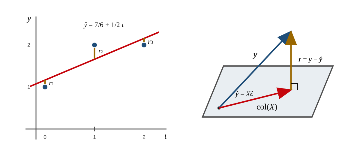
Figure 4.3.9. Two views of the same line fit. In the data plot, the residuals are vertical differences \(r_i=y_i-\widehat y_i\text{.}\) In \(\mathbb{R}^3\text{,}\) the fitted vector \(\widehat{\mathbf{y}}=X\widehat{\mathbf{c}}\) is the projection of \(\mathbf{y}\) onto \(\operatorname{col}(X)\text{,}\) and \(\mathbf{r}\perp\operatorname{col}(X)\text{.}\) The two panels in
the figure 4.3.9 show different spaces: the left panel is the
\(t\) -
\(y\) data plot, while the right panel is the output space
\(\mathbb{R}^3\text{.}\)
Activity 4.3.10 . Reading regression code (U4-LO4, U4-LO7).
import numpy as np

t = np.array([0.0, 1.0, 2.0])
y = np.array([1.0, 2.0, 2.0])

X = np.column_stack([np.ones_like(t), t])

c = np.linalg.lstsq(X, y, rcond=None)[0]
yhat = X @ c
r = y - yhat

X, c, yhat, r, X.T @ r, np.linalg.norm(r)**2
What array is produced by
np.ones_like(t)?
What does
np.column_stack([np.ones_like(t), t]) construct?
What does
[0] select from the value returned by
np.linalg.lstsq?
Why does
c have two entries?
What mathematical objects are stored in
yhat and
r?
Why is the residual check
X.T @ r rather than
X @ r?
What should
X.T @ r be close to?
Does a nonzero residual vector mean the code failed?
What quantity is computed by
np.linalg.norm(r)**2?
Solution .
np.column_stack([np.ones_like(t), t])
uses those two arrays as columns, so
\begin{equation*}
X
=
\begin{bmatrix}
1\amp0\\
1\amp1\\
1\amp2
\end{bmatrix}.
\end{equation*}
The function
np.linalg.lstsq returns several objects. The index
[0] selects the least-squares coefficient vector. The vector
c has two entries because the design matrix has two columns: one for the constant feature and one for the
\(t\) -feature.
The variable yhat stores the fitted vector
\begin{equation*}
\widehat{\mathbf{y}}
=
X\widehat{\mathbf{c}},
\end{equation*}
and r stores the residual vector
\begin{equation*}
\mathbf{r}
=
\mathbf{y}-\widehat{\mathbf{y}}.
\end{equation*}
The product
X.T @ r computes dot products with the columns of
\(X\text{.}\) It checks that the residual is orthogonal to the column space. The product
X @ r is not the correct operation and does not have compatible shapes in this example.
The output
X.T @ r should be close to
A nonzero residual does not mean the code failed. The data vector is not exactly in the column space, so the closest fit has a nonzero residual.
computes the sum of squared residuals. Its value is
\begin{equation*}
\frac{1}{6}
\end{equation*}
up to roundoff.