Orthogonal projection

Section 4.2 Orthogonal projection

Subsection Orthogonal complements and projections

Definition 4.2.1. The orthogonal complement of a subspace.

If \(U\) is a subspace of \(\R^n\text{,}\) the orthogonal complement of \(U\) is the subset of \(\R^n\) given by

\begin{equation*} U^\perp = \{\mathbf{x} \text{ in } \R^n \mid \mathbf{x} \cdot \mathbf{y} = 0 \text{ for all } \mathbf{y} \text{ in } U\} \end{equation*}

🔗

Theorem 4.2.2.

The following properties of the orthogonal complement hold:

For any subspace \(U\) of \(\R^n\text{,}\) \(U^\perp\) is a subspace of \(\R^n\)

🔗
\(\{0\}^\perp = \R^n\) and \((\R^n)^\perp = \{0\}\)

🔗
If \(U = \spans \{\mathbf{x}_1,\ldots,\mathbf{x}_k\}\text{,}\) then
\begin{equation*} U^\perp = \{\mathbf{x} \text{ in } \R^n \mid \mathbf{x} \cdot \mathbf{x}_i = 0 \text{ for } i=1,2,\ldots,k\} \end{equation*}

🔗

🔗

Activity 4.2.3. Finding an orthogonal complement (U4-LO2).

Find \(U^\perp\) if \(U = \spans \{(1,1,0), (0,1,1)\}\) in \(\R^3\text{.}\)

🔗

Solution.

The third property of Theorem 4.2.2 implies that a vector \(\mathbf{w} = (x,y,z)\) lies in \(U^\perp\) if and only if it is orthogonal to both \((1,1,0)\) and \((0,1,1)\text{.}\) Taking these two dot products gives

\begin{align*} \mathbf{w}\cdot(1,1,0)=x+y \amp = 0\\ \mathbf{w}\cdot(0,1,1)=y+z \amp = 0. \end{align*}

From \(x+y=0\text{,}\) we obtain \(x=-y\text{.}\) From \(y+z=0\text{,}\) we obtain \(z=-y\text{.}\) The variable \(y\) is free, so every solution can be written as

\begin{equation*} \mathbf{w}=(-y,y,-y)=y(-1,1,-1), \qquad y\in\R. \end{equation*}

Thus every vector in \(U^\perp\) is a multiple of \((-1,1,-1)\text{,}\) and

\begin{equation*} U^\perp = \spans \left\{ \begin{bmatrix}-1\\1\\-1\end{bmatrix} \right\} = \left\{ \begin{bmatrix}-y\\y\\-y\end{bmatrix}: y \in \R \right\} \text{.} \end{equation*}

🔗

Lemma 4.2.4. Expanding an orthogonal set.

Let \(\{\mathbf{f}_1, \mathbf{f}_2, \ldots, \mathbf{f}_m\}\) be an orthogonal set in \(\R^n\text{.}\) Given \(\mathbf{x}\) in \(\R^n\text{,}\) write

\begin{equation*} \mathbf{f}_{m+1} = \mathbf{x} - \frac{\mathbf{x}\cdot\mathbf{f}_1}{\|\mathbf{f}_1\|^2}\mathbf{f}_1 - \frac{\mathbf{x}\cdot\mathbf{f}_2}{\|\mathbf{f}_2\|^2}\mathbf{f}_2 - \cdots - \frac{\mathbf{x}\cdot\mathbf{f}_m}{\|\mathbf{f}_m\|^2}\mathbf{f}_m \end{equation*}

Then:

\(\mathbf{f}_{m+1} \cdot \mathbf{f}_k = 0\) for \(k = 1,2,\ldots,m\)

🔗
If \(\mathbf{x} \not \in \spans \{\mathbf{f}_1,\ldots,\mathbf{f}_m\}\text{,}\) then \(\mathbf{f}_{m+1} \neq \mathbf{0}\) and \(\{\mathbf{f}_1,\ldots,\mathbf{f}_m,\mathbf{f}_{m+1}\}\) is an orthogonal set.

🔗

🔗

Why is this true?.

For convenience, let \(t_i = \frac{\mathbf{x} \cdot \mathbf{f}_i}{\|\mathbf{f}_i\|^2}\) for each \(i\text{.}\) Given \(1 \leq k \leq m\text{,}\) we calculate that

\begin{align*} \mathbf{f}_{m+1} \cdot \mathbf{f}_k \amp = (\mathbf{x} - t_1\mathbf{f}_1 - t_2\mathbf{f}_2 - \cdots - t_m\mathbf{f}_m) \cdot \mathbf{f}_k\\ \amp = \mathbf{x} \cdot \mathbf{f}_k - t_1(\mathbf{f}_1 \cdot \mathbf{f}_k) - \cdots - t_k(\mathbf{f}_k \cdot \mathbf{f}_k) - \cdots - t_m(\mathbf{f}_m \cdot \mathbf{f}_k) \end{align*}

Since \(\{\mathbf{f}_1, \mathbf{f}_2, \ldots, \mathbf{f}_m\}\) is an orthogonal set, \(\mathbf{f}_i \cdot \mathbf{f}_k = 0\) for all \(i \neq k\text{.}\) So

\begin{align*} \mathbf{f}_{m+1} \cdot \mathbf{f}_k \amp = \mathbf{x} \cdot \mathbf{f}_k - t_k(\mathbf{f}_k \cdot \mathbf{f}_k)\\ \amp = \mathbf{x} \cdot \mathbf{f}_k - \frac{\mathbf{x} \cdot \mathbf{f}_k}{\|\mathbf{f}_k\|^2} \cdot \|\mathbf{f}_k\|^2\\ \amp = \mathbf{x} \cdot \mathbf{f}_k - \mathbf{x} \cdot \mathbf{f}_k = 0 \end{align*}

This proves the first property of the lemma. To prove the second, we note that if \(\mathbf{f}_{m+1}\) was zero, then \(\mathbf{x}\) would be in the span of the vectors \(\{\mathbf{f}_1,\ldots,\mathbf{f}_m\}\text{.}\) So if \(\mathbf{x}\) is not in the span, then \(\mathbf{f}_{m+1}\) can not be equal to zero. And we have proved \(\mathbf{f}_{m+1}\) is orthogonal to the vectors \(\mathbf{f}_1, \dots, \mathbf{f}_m\text{,}\) so that \(\{ \mathbf{f}_1, \dots, \mathbf{f}_{m+1} \}\) is an orthogonal set.

🔗

Activity 4.2.5. Extending an orthogonal set to a basis (U4-LO2).

Use Lemma 4.2.4 to extend the orthogonal set \(\{ \mathbf{f}_1, \mathbf{f}_2 \}\) in \(\R^3\) to an orthogonal basis \(\{ \mathbf{f}_1, \mathbf{f}_2, \mathbf{f}_3 \}\text{,}\) where

\begin{equation*} \mathbf{f}_1 = \begin{bmatrix}1\\1\\0\end{bmatrix} \quad\text{and}\quad \mathbf{f}_2 = \begin{bmatrix}1\\-1\\0\end{bmatrix}\text{,} \end{equation*}

using the vector \(\mathbf{x} = (1,1,2)\) as in that lemma.

🔗

Solution.

We calculate that

\begin{align*} \mathbf{x} \cdot \mathbf{f}_1 \amp = (1,1,2) \cdot (1,1,0) = 1 + 1 + 0 = 2\\ \|\mathbf{f}_1\|^2 \amp = 1^2 + 1^2 + 0^2 = 2\\ \mathbf{x} \cdot \mathbf{f}_2 \amp = (1,1,2) \cdot (1,-1,0) = 1 - 1 + 0 = 0\\ \|\mathbf{f}_2\|^2 \amp = 1^2 + (-1)^2 + 0^2 = 2 \end{align*}

Using Lemma 4.2.4, we define

\begin{align*} \mathbf{f}_3 \amp = \mathbf{x} - \frac{\mathbf{x} \cdot \mathbf{f}_1}{\|\mathbf{f}_1\|^2}\mathbf{f}_1 - \frac{\mathbf{x} \cdot \mathbf{f}_2}{\|\mathbf{f}_2\|^2}\mathbf{f}_2\\ \amp = \begin{bmatrix}1\\1\\2\end{bmatrix} - \frac{2}{2}\begin{bmatrix}1\\1\\0\end{bmatrix} - \frac{0}{2}\begin{bmatrix}1\\-1\\0\end{bmatrix} = \begin{bmatrix}0\\0\\2\end{bmatrix}\text{.} \end{align*}

🔗

Definition 4.2.6. The orthogonal projection onto a subspace.

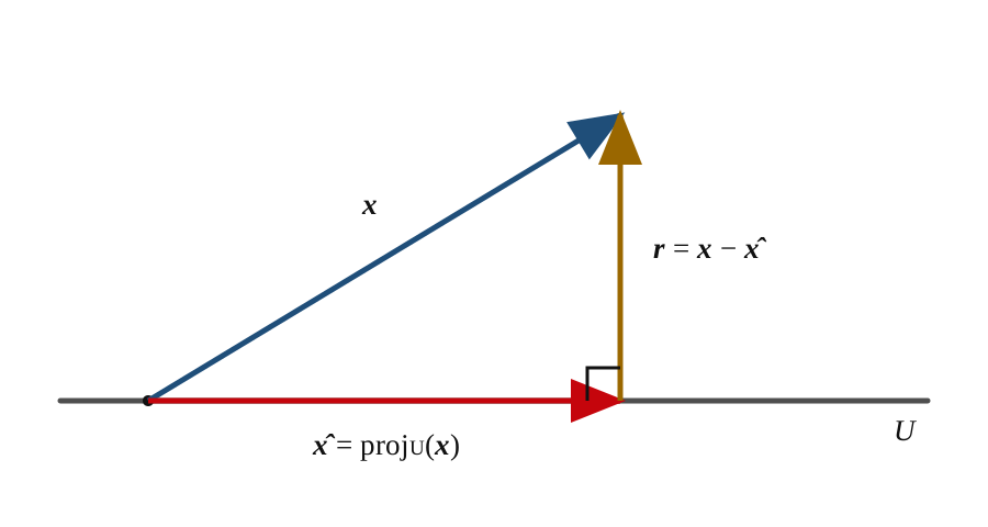
Let \(U\) be a subspace of \(\R^n\text{.}\) Then the orthogonal projection of the vector \(\mathbf{x} \in \R^n\) onto \(U\) is the vector \(\mathbf{y}=\proj_U(\mathbf{x}) \in U\) which is closest to \(\mathbf{x}\text{,}\) in the sense that for any \(\mathbf{z} \in U\) with \(\mathbf{z} \neq \mathbf{y}\text{,}\) \(\| \mathbf{x} - \mathbf{y} \| \lt \| \mathbf{x} - \mathbf{z} \|\text{.}\) The residual is the difference between the original vector and its projection:

\begin{equation*} \mathbf{r}=\mathbf{x}-\mathbf{y}=\mathbf{x}-\proj_U(\mathbf{x}). \end{equation*}

🔗

Orthogonal projection decomposes the original vector into a vector in the subspace and a residual perpendicular to the subspace.

🔗

A vector x is decomposed into its projection x-hat along the subspace U and a perpendicular residual r. A right-angle marker shows that the residual is orthogonal to U. — Figure 4.2.7. Projection and residual. Orthogonal projection writes \(\mathbf{x}=\widehat{\mathbf{x}}+\mathbf{r}\text{,}\) where \(\widehat{\mathbf{x}}\in U\) and \(\mathbf{r}\in U^\perp\text{.}\)
🔗

The following theorem gives us a practical way to calculate orthogonal projections.

🔗

Theorem 4.2.8. Projection theorem.

Let \(U\) be a subspace of \(\R^n\) with orthogonal basis \(\{\mathbf{f}_1,\ldots,\mathbf{f}_m\}\text{.}\) For any vector \(\mathbf{x} \in \R^n\text{,}\) define

\begin{equation*} \mathbf{y} = \frac{\mathbf{x}\cdot\mathbf{f}_1}{\|\mathbf{f}_1\|^2}\mathbf{f}_1 + \frac{\mathbf{x}\cdot\mathbf{f}_2}{\|\mathbf{f}_2\|^2}\mathbf{f}_2 + \cdots + \frac{\mathbf{x}\cdot\mathbf{f}_m}{\|\mathbf{f}_m\|^2}\mathbf{f}_m. \end{equation*}

Then \(\mathbf{y}=\proj_U(\mathbf{x})\text{.}\) The residual

\begin{equation*} \mathbf{r}=\mathbf{x}-\mathbf{y}=\mathbf{x}-\proj_U(\mathbf{x}) \end{equation*}

lies in \(U^\perp\text{.}\) In particular, if \(\mathbf{x}\) is already in \(U\text{,}\) then \(\mathbf{x}\) equals the displayed sum.

🔗

Why is this true?.

If \(\{ \mathbf{f}_1, \dots, \mathbf{f}_m \}\) is an orthogonal basis for \(U\text{,}\) and we define

\begin{equation*} \mathbf{y} = \frac{\mathbf{x} \cdot \mathbf{f}_1}{\|\mathbf{f}_1\|^2}\mathbf{f}_1 + \frac{\mathbf{x} \cdot \mathbf{f}_2}{\|\mathbf{f}_2\|^2}\mathbf{f}_2 + \cdots + \frac{\mathbf{x} \cdot \mathbf{f}_m}{\|\mathbf{f}_m\|^2}\mathbf{f}_m\text{,} \end{equation*}

then \(\mathbf{y}\) is evidently a linear combination of the basis \(\{ \mathbf{f}_1, \dots, \mathbf{f}_m \}\text{,}\) so \(\mathbf{y} \in U\text{.}\) And Lemma 4.2.4 states that \(\mathbf{x} - \mathbf{y} \in U^\perp\text{.}\) Thus if \(\mathbf{z} \in U\) and \(\mathbf{z} \neq \mathbf{y}\text{,}\) the Pythagorean theorem (Theorem 4.1.11) tells us that

\begin{align*} \| \mathbf{x} - \mathbf{z} \|^2 \amp = \| (\mathbf{x} - \mathbf{y}) + (\mathbf{y} - \mathbf{z}) \|^2\\ \amp = \| \mathbf{x} - \mathbf{y} \|^2 + \| \mathbf{y} - \mathbf{z} \|^2\text{.} \end{align*}

Since \(\mathbf{y} \neq \mathbf{z}\text{,}\) we find that

\begin{equation*} \| \mathbf{x} - \mathbf{z} \|^2 \gt \| \mathbf{x} - \mathbf{y} \|^2\text{,} \end{equation*}

and taking square roots gives that

\begin{equation*} \| \mathbf{x} - \mathbf{z} \| \gt \| \mathbf{x} - \mathbf{y} \|\text{.} \end{equation*}

Thus the vector \(\mathbf{y}\) we have defined is equal to \(\proj_U(\mathbf{x})\text{.}\) Since we have already verified that \(\mathbf{x} - \mathbf{y} = \mathbf{x} - \proj_U(\mathbf{x})\) is in \(U^\perp\text{,}\) the theorem follows.

🔗

Activity 4.2.9. Projecting onto a span (U4-LO3).

Find \(\proj_U \mathbf{x}\) where \(U = \spans \{(1,1,0), (1,-1,0)\}\) and \(\mathbf{x} = (2,0,1)\) in \(\R^3\text{.}\)

🔗

Solution.

The vectors \(\mathbf{f}_1 = (1,1,0)\) and \(\mathbf{f}_2 = (1,-1,0)\) are already orthogonal, as

\begin{equation*} \mathbf{f}_1 \cdot \mathbf{f}_2 = 1 \cdot 1 + 1 \cdot (-1) + 0 \cdot 0 = 0\text{.} \end{equation*}

They thus form an orthogonal basis for \(U\text{.}\) We calculate the following values:

\begin{align*} \mathbf{x} \cdot \mathbf{f}_1 \amp = (2,0,1) \cdot (1,1,0)\\ \amp = 2 \cdot 1 + 0 \cdot 1 + 1 \cdot 0 = 2\\ \|\mathbf{f}_1\|^2 \amp = 1^2 + 1^2 + 0^2 = 2\\ \mathbf{x} \cdot \mathbf{f}_2 \amp = (2,0,1) \cdot (1,-1,0)\\ \amp = 2 \cdot 1 + 0 \cdot (-1) + 1 \cdot 0 = 2\\ \|\mathbf{f}_2\|^2 \amp = 1^2 + (-1)^2 + 0^2 = 2 \end{align*}

Using Theorem 4.2.8, we calculate that

\begin{align*} \proj_U \mathbf{x} \amp = \frac{\mathbf{x} \cdot \mathbf{f}_1}{\|\mathbf{f}_1\|^2}\mathbf{f}_1 + \frac{\mathbf{x} \cdot \mathbf{f}_2}{\|\mathbf{f}_2\|^2}\mathbf{f}_2\\ \amp = \frac{2}{2}\begin{bmatrix}1\\1\\0\end{bmatrix} + \frac{2}{2}\begin{bmatrix}1\\-1\\0\end{bmatrix} = \begin{bmatrix}2\\0\\0\end{bmatrix}\text{.} \end{align*}

🔗

Activity 4.2.10. Projection onto a line (U4-LO3).

Let

\begin{equation*} \mathbf{u}=\begin{bmatrix}3\\4\end{bmatrix},\qquad \mathbf{x}=\begin{bmatrix}2\\5\end{bmatrix},\qquad L=\operatorname{span}\{\mathbf{u}\}. \end{equation*}

🔗

Compute \(\operatorname{proj}_L(\mathbf{x})\text{.}\)
🔗

🔗
Compute the residual \(\mathbf{r}=\mathbf{x}-\operatorname{proj}_L(\mathbf{x})\text{.}\)
🔗

🔗
Check that \(\mathbf{r}\cdot\mathbf{u}=0\text{.}\)
🔗

🔗

Solution.

We have \(\mathbf{x}\cdot\mathbf{u}=26\) and \(\mathbf{u}\cdot\mathbf{u}=25\text{.}\) Therefore

\begin{equation*} \operatorname{proj}_L(\mathbf{x}) = \frac{\mathbf{x}\cdot\mathbf{u}}{\mathbf{u}\cdot\mathbf{u}}\mathbf{u} = \frac{26}{25}\begin{bmatrix}3\\4\end{bmatrix} = \begin{bmatrix}78/25\\104/25\end{bmatrix}. \end{equation*}

The residual is

\begin{equation*} \mathbf{r} = \begin{bmatrix}2\\5\end{bmatrix} - \begin{bmatrix}78/25\\104/25\end{bmatrix} = \begin{bmatrix}-28/25\\21/25\end{bmatrix}. \end{equation*}

Finally,

\begin{equation*} \mathbf{r}\cdot\mathbf{u} = \left(-\frac{28}{25}\right)3+\left(\frac{21}{25}\right)4 = 0. \end{equation*}

🔗

Activity 4.2.11. Projection onto a line in code (U4-LO3, U4-LO7).

The following code computes the same projection and residual as the previous activity.

🔗

import numpy as np

u = np.array([3.0, 4.0])
x = np.array([2.0, 5.0])

y = (x @ u) / (u @ u) * u
r = x - y

y, r, r @ u

Which variable stores the projection?
🔗

🔗
Which variable stores the residual?
🔗

🔗
Why should r @ u be close to zero?
🔗

🔗
What does (x @ u) / (u @ u) * u compute?
🔗

🔗

Solution.

The variable y stores the projection and r stores the residual. The value r @ u checks whether the residual is orthogonal to the direction of the line, so it should be close to zero. The expression (x @ u) / (u @ u) * u computes the orthogonal projection of \(\mathbf{x}\) onto \(L=\spans\{\mathbf{u}\}\text{:}\)

\begin{equation*} \proj_L(\mathbf{x})=\frac{\mathbf{x}\cdot\mathbf{u}}{\mathbf{u}\cdot\mathbf{u}}\mathbf{u}. \end{equation*}

🔗

Directional derivatives as projection coefficients.

Let \(\mathbf v\) be a unit vector. By Theorem 4.2.8,

\begin{equation*} \operatorname{proj}_{\operatorname{span}\{\mathbf v\}}\bigl(\nabla f(\mathbf a)\bigr)=\bigl(\nabla f(\mathbf a)\cdot\mathbf v\bigr)\mathbf v. \end{equation*}

By Theorem 3.6.3,

\begin{equation*} \operatorname{proj}_{\operatorname{span}\{\mathbf v\}}\bigl(\nabla f(\mathbf a)\bigr)=D_{\mathbf v}f(\mathbf a)\mathbf v. \end{equation*}

Thus \(D_{\mathbf v}f(\mathbf a)\) is the signed projection coefficient of the gradient in the oriented direction \(\mathbf v\text{.}\) Its absolute value is the length of the projection. The Cauchy–Schwarz inequality in Theorem 4.1.2 gives

\begin{equation*} |D_{\mathbf v}f(\mathbf a)|\leq\|\nabla f(\mathbf a)\|. \end{equation*}

🔗

Activity 4.2.12. Directional derivative as a projection coefficient (U4-LO3, U3-LO8).

Reopen Activity 3.6.4. For each listed unit vector \(\mathbf v_i\text{,}\) compute

\begin{equation*} \operatorname{proj}_{\operatorname{span}\{\mathbf v_i\}}\bigl(\nabla f(\mathbf a)\bigr)=D_{\mathbf v_i}f(\mathbf a)\mathbf v_i. \end{equation*}

🔗

Which projection coefficients are positive, and which are negative?
🔗

🔗
Why do \(\mathbf v_3\) and \(\mathbf v_4\) give the same projection vector but opposite directional derivatives?
🔗

🔗
Reopen Figure 3.6.9. How does the figure distinguish greatest increase, greatest decrease, and zero change?
🔗

🔗

Solution.

From Activity 3.6.4,

\begin{align*} D_{\mathbf v_1}f(\mathbf a)\amp=3,\qquad D_{\mathbf v_2}f(\mathbf a)=4,\\ D_{\mathbf v_3}f(\mathbf a)\amp=5,\qquad D_{\mathbf v_4}f(\mathbf a)=-5. \end{align*}

Therefore,

\begin{equation*} \operatorname{proj}_{\operatorname{span}\{\mathbf v_1\}}\bigl(\nabla f(\mathbf a)\bigr)=3\mathbf v_1=\begin{bmatrix}3\\0\end{bmatrix}, \end{equation*}

\begin{equation*} \operatorname{proj}_{\operatorname{span}\{\mathbf v_2\}}\bigl(\nabla f(\mathbf a)\bigr)=4\mathbf v_2=\begin{bmatrix}0\\4\end{bmatrix}, \end{equation*}

and

\begin{equation*} \operatorname{proj}_{\operatorname{span}\{\mathbf v_3\}}\bigl(\nabla f(\mathbf a)\bigr)=5\mathbf v_3=\begin{bmatrix}3\\4\end{bmatrix}. \end{equation*}

Since \(\mathbf v_4=-\mathbf v_3\text{,}\)

\begin{equation*} \operatorname{proj}_{\operatorname{span}\{\mathbf v_4\}}\bigl(\nabla f(\mathbf a)\bigr)=(-5)\mathbf v_4=\begin{bmatrix}3\\4\end{bmatrix}. \end{equation*}

The vectors \(\mathbf v_3\) and \(\mathbf v_4\) span the same line, so projection onto that line gives the same vector. The directional derivatives have opposite signs because the two unit vectors give opposite orientations of the line. Figure 3.6.9 shows greatest increase in the gradient direction, greatest decrease in the opposite direction, and zero change in directions orthogonal to the gradient.

🔗

Projection as an optimization problem.

Orthogonal projection can also be described by minimizing a distance function.

🔗

Example 4.2.13.

A common optimization problem that we have already encountered in Definition 4.2.6 involves taking a subspace \(U \subseteq \R^n\) and a given vector \(\mathbf{x}_0 \in \R^n\text{,}\) and finding the vector \(\mathbf{x}^* \in U\) that is closest to \(\mathbf{x}_0\text{,}\) i.e., finding the vector that minimizes the scalar-valued function \(g: \R^n \to \R\) on \(U\text{,}\) defined by setting \(g(\mathbf{x}) = \| \mathbf{x}_0 - \mathbf{x} \|\text{.}\) Then \(\mathbf{x}^*\) is the orthogonal projection of \(\mathbf{x}_0\) onto \(U\text{,}\) and we have seen in Theorem 4.2.8 that if \(U\) has an orthogonal basis \(\{ \mathbf{f}_1, \dots, \mathbf{f}_m \}\text{,}\) then

\begin{equation*} \mathbf{x}^* = \frac{\mathbf{x}_0\cdot\mathbf{f}_1}{\|\mathbf{f}_1\|^2}\mathbf{f}_1 + \frac{\mathbf{x}_0\cdot\mathbf{f}_2}{\|\mathbf{f}_2\|^2}\mathbf{f}_2 + \cdots + \frac{\mathbf{x}_0\cdot\mathbf{f}_m}{\|\mathbf{f}_m\|^2}\mathbf{f}_m. \end{equation*}

In Section 5.6, we return to this viewpoint and derive the normal equations by setting a gradient equal to zero.

🔗

Activity 4.2.14. Projection as optimization (U4-LO3, U3-LO9).

Let

\begin{equation*} W=\operatorname{span}\left\{ \begin{bmatrix} 1\\ 0 \end{bmatrix} \right\} \subseteq \mathbb{R}^2, \qquad \mathbf{b}= \begin{bmatrix} 2\\ 3 \end{bmatrix}. \end{equation*}

A general point of \(W\) has the form

\begin{equation*} \mathbf{w}(t)= \begin{bmatrix} t\\ 0 \end{bmatrix}. \end{equation*}

🔗

Write the squared distance \(g(t)=\|\mathbf{b}-\mathbf{w}(t)\|^2\text{.}\)
🔗

🔗
Compute \(g'(t)\) and find the critical point of \(g\text{.}\)
🔗

🔗
Use \(g''(t)\) to classify the critical point.
🔗

🔗
What point of \(W\) is closest to \(\mathbf{b}\text{?}\)
🔗

🔗
How does this agree with Figure 4.2.7 and Theorem 4.2.8?
🔗

🔗

Solution.

We have

\begin{equation*} \mathbf{b}-\mathbf{w}(t)= \begin{bmatrix} 2-t\\ 3 \end{bmatrix}, \end{equation*}

\begin{equation*} g(t)=\|\mathbf{b}-\mathbf{w}(t)\|^2=(2-t)^2+9. \end{equation*}

Differentiating gives

\begin{equation*} g'(t)=2(t-2). \end{equation*}

The unique critical point is \(t=2\text{.}\) Since

\begin{equation*} g''(t)=2>0, \end{equation*}

this critical point is a local minimum. Because \(g\) is an upward-opening quadratic, it is also the unique global minimum. Therefore the closest point in \(W\) is

\begin{equation*} \hat{\mathbf{b}}= \begin{bmatrix} 2\\ 0 \end{bmatrix}. \end{equation*}

This agrees with Figure 4.2.7 and Theorem 4.2.8: the residual is

\begin{equation*} \mathbf{b}-\hat{\mathbf{b}}= \begin{bmatrix} 0\\ 3 \end{bmatrix}. \end{equation*}

For every \(\mathbf{w}(t)\in W\text{,}\)

\begin{equation*} (\mathbf{b}-\hat{\mathbf{b}})\cdot\mathbf{w}(t) = \begin{bmatrix} 0\\ 3 \end{bmatrix} \cdot \begin{bmatrix} t\\ 0 \end{bmatrix} =0\cdot t+3\cdot 0=0. \end{equation*}

Therefore the residual is orthogonal to \(W\text{.}\)

🔗

Connection: score, then combine.

Projection and attention both use dot products to score directions and then use the resulting numbers in a linear combination.

🔗

Let

\begin{equation*} Q= \begin{bmatrix} \mathbf{q}_1\amp\cdots\amp\mathbf{q}_k \end{bmatrix} \end{equation*}

have orthonormal columns. Then

\begin{equation*} Q^T\mathbf{x} = \begin{bmatrix} \mathbf{q}_1^T\mathbf{x}\\ \vdots\\ \mathbf{q}_k^T\mathbf{x} \end{bmatrix} \end{equation*}

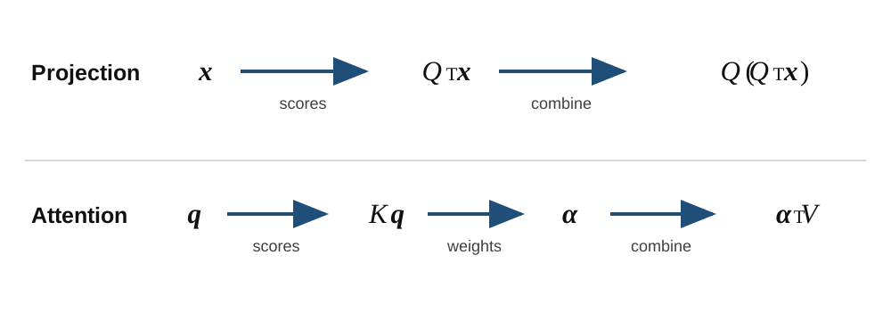
collects the directional coefficients of \(\mathbf{x}\text{.}\) Because each \(\mathbf{q}_i\) has length \(1\text{,}\) these dot products are the coordinates used in the projection. If \(\mathbf{x}\) also has length \(1\text{,}\) they are cosine similarities with the directions \(\mathbf{q}_i\text{.}\)

🔗

Multiplying by \(Q\) combines the directions using those coefficients:

\begin{equation*} Q(Q^T\mathbf{x}) = \sum_{i=1}^k (\mathbf{q}_i^T\mathbf{x})\mathbf{q}_i = \operatorname{proj}_{\operatorname{col}(Q)}(\mathbf{x}). \end{equation*}

🔗

Thus projection follows the pattern

\begin{equation*} \text{score with }Q^T \quad\longrightarrow\quad \text{combine with }Q. \end{equation*}

🔗

Two parallel pipelines. Projection sends x to Q transpose x and then to Q times Q transpose x. Attention sends a query q to Kq, then to weights alpha, and then to alpha transpose V. — Figure 4.2.15. Score, then combine. Projection uses \(Q^T\mathbf{x}\) to score orthonormal directions and \(Q(Q^T\mathbf{x})\) to combine them. Attention uses query-key scores, converts them into weights, and combines value vectors.
🔗

Attention has the same broad pattern. Query-key dot products produce scores, a weighting rule converts the scores into weights, and the weights combine value vectors. Projection scores and combines the same orthonormal directions. Attention scores key vectors and then combines value vectors, which may be different vectors. Projection also chooses its coefficients so that the residual is orthogonal to the subspace. Attention is therefore not generally an orthogonal projection, but both computations are built from dot products and linear combinations.

🔗

Activity 4.2.16. Dot-product scores as projection coordinates (U4-LO1, U4-LO3).

Let

\begin{equation*} \mathbf{q}_1 = \frac{1}{\sqrt{2}} \begin{bmatrix} 1\\ 1\\ 0 \end{bmatrix}, \qquad \mathbf{q}_2 = \frac{1}{\sqrt{2}} \begin{bmatrix} 1\\ -1\\ 0 \end{bmatrix}, \qquad \mathbf{x} = \begin{bmatrix} 2\\ 0\\ 1 \end{bmatrix}, \end{equation*}

and let

\begin{equation*} Q= \begin{bmatrix} \mathbf{q}_1\amp\mathbf{q}_2 \end{bmatrix}. \end{equation*}

🔗

Verify that the columns of \(Q\) are orthonormal.
🔗

🔗
Compute the score vector

\begin{equation*} \mathbf{c}=Q^T\mathbf{x}. \end{equation*}

🔗

🔗
Compute

\begin{equation*} \widehat{\mathbf{x}}=Q\mathbf{c}. \end{equation*}

🔗

🔗
Compute the residual

\begin{equation*} \mathbf{r}=\mathbf{x}-\widehat{\mathbf{x}}, \end{equation*}

and verify that \(Q^T\mathbf{r}=\mathbf{0}\text{.}\)

🔗

🔗
Explain why the entries of \(\mathbf{c}\) can be read both as dot-product scores and as coordinates of the projection.
🔗

🔗
Explain how the calculation follows the pattern “score, then combine.” What extra condition identifies \(\widehat{\mathbf{x}}\) as an orthogonal projection?
🔗

🔗

Solution.

The two columns have length \(1\text{,}\) and

\begin{equation*} \mathbf{q}_1^T\mathbf{q}_2 = \frac{1}{2}(1-1)=0. \end{equation*}

Thus the columns of \(Q\) are orthonormal.

🔗

The score vector is

\begin{equation*} \mathbf{c} = Q^T\mathbf{x} = \begin{bmatrix} \mathbf{q}_1^T\mathbf{x}\\ \mathbf{q}_2^T\mathbf{x} \end{bmatrix} = \begin{bmatrix} \sqrt{2}\\ \sqrt{2} \end{bmatrix}. \end{equation*}

🔗

Combining the columns of \(Q\) using these scores gives

\begin{equation*} \widehat{\mathbf{x}} = Q\mathbf{c} = \sqrt{2}\mathbf{q}_1+\sqrt{2}\mathbf{q}_2 = \begin{bmatrix} 2\\ 0\\ 0 \end{bmatrix}. \end{equation*}

🔗

The residual is

\begin{equation*} \mathbf{r} = \mathbf{x}-\widehat{\mathbf{x}} = \begin{bmatrix} 0\\ 0\\ 1 \end{bmatrix}. \end{equation*}

🔗

Therefore

\begin{equation*} Q^T\mathbf{r} = \begin{bmatrix} 0\\ 0 \end{bmatrix}. \end{equation*}

🔗

Each entry of \(\mathbf{c}\) is a dot product with one of the unit directions, so it is both a directional score and a coordinate used to reconstruct the projection. The calculation first scores \(\mathbf{x}\) with \(Q^T\text{,}\) then combines the columns of \(Q\) using those scores. The condition \(Q^T\mathbf{r}=\mathbf{0}\) says that the residual is orthogonal to every column of \(Q\text{.}\) This is the extra condition that identifies \(\widehat{\mathbf{x}}\) as the orthogonal projection.

🔗

Subsection Gram-Schmidt orthogonalization

Gram-Schmidt is a sequence of projection, subtraction, measurement, and normalization steps. Use Perfectly Normal to practice the same sequence geometrically. The game uses an original column \(\mathbf{a}_j\text{,}\) its projection \(\mathbf{p}_j\text{,}\) the residual \(\mathbf{v}_j\text{,}\) the new unit direction \(\mathbf{q}_j\text{,}\) and coefficients \(r_{ij}\text{.}\)

🔗

Algorithm 4.2.17. Gram-Schmidt algorithm.

Input: A matrix

\begin{equation*} A= \begin{bmatrix} \mathbf{a}_1 \amp \mathbf{a}_2 \amp \cdots \amp \mathbf{a}_n \end{bmatrix} \end{equation*}

with linearly independent columns.

🔗

For \(j=1,\ldots,n\text{:}\)

🔗

Current column. Start with \(\mathbf{a}_j\text{.}\)
🔗

🔗
Project. For each \(i \lt j\text{,}\) compute

\begin{equation*} r_{ij}=\mathbf{q}_i^T\mathbf{a}_j. \end{equation*}

Then assemble

\begin{equation*} \mathbf{p}_j=\sum_{i \lt j}r_{ij}\mathbf{q}_i. \end{equation*}

For the first column, \(\mathbf{p}_1=\mathbf{0}\text{.}\)

🔗

🔗
Subtract.

\begin{equation*} \mathbf{v}_j=\mathbf{a}_j-\mathbf{p}_j. \end{equation*}

🔗

🔗
Measure.

\begin{equation*} r_{jj}=\|\mathbf{v}_j\|. \end{equation*}

🔗

🔗
Normalize.

\begin{equation*} \mathbf{q}_j=\frac{\mathbf{v}_j}{r_{jj}}. \end{equation*}

🔗

🔗

Output: The vectors \(\mathbf{q}_1,\ldots,\mathbf{q}_n\) are orthonormal, and

\begin{equation*} \spans\{\mathbf{q}_1,\ldots,\mathbf{q}_j\} = \spans\{\mathbf{a}_1,\ldots,\mathbf{a}_j\} \end{equation*}

at every stage.

🔗

Warning 4.2.18.

If \(r_{jj}=0\text{,}\) then \(\mathbf{a}_j\) is already in the span of the earlier columns. The input columns are not linearly independent, and no new unit direction is produced.

🔗

The same algorithm in orthogonal form. Repeatedly applying Lemma 4.2.4 gives the theorem below. The theorem first constructs orthogonal residuals \(\mathbf{f}_j\text{,}\) while the algorithm above normalizes each residual to obtain \(\mathbf{q}_j\text{.}\) The two forms agree because

\begin{equation*} \mathbf{q}_i=\frac{\mathbf{f}_i}{\|\mathbf{f}_i\|} \end{equation*}

and

\begin{equation*} \frac{\mathbf{a}_j^T\mathbf{f}_i}{\|\mathbf{f}_i\|^2}\mathbf{f}_i = (\mathbf{q}_i^T\mathbf{a}_j)\mathbf{q}_i. \end{equation*}

🔗

Theorem 4.2.19. The Gram-Schmidt orthogonalization algorithm.

Let \(U\) be a subspace of \(\R^n\text{.}\) Then \(U\) has an orthogonal basis.

🔗

Given a basis \(\{ \mathbf{x}_1, \dots, \mathbf{x}_m \}\) of \(U\text{,}\) we can iteratively define an orthogonal basis \(\{ \mathbf{f}_1, \dots, \mathbf{f}_m \}\) of \(U\) by defining

\begin{align*} \mathbf{f}_1 \amp = \mathbf{x}_1\\ \mathbf{f}_2 \amp = \mathbf{x}_2 - \frac{\mathbf{x}_2 \cdot \mathbf{f}_1}{\|\mathbf{f}_1\|^2}\mathbf{f}_1\\ \mathbf{f}_3 \amp = \mathbf{x}_3 - \frac{\mathbf{x}_3 \cdot \mathbf{f}_1}{\|\mathbf{f}_1\|^2}\mathbf{f}_1 - \frac{\mathbf{x}_3 \cdot \mathbf{f}_2}{\|\mathbf{f}_2\|^2}\mathbf{f}_2 \end{align*}

and so on, i.e., for \(2 \leq k \leq m\) defining

\begin{equation*} \mathbf{f}_k = \mathbf{x}_k - \frac{\mathbf{x}_k \cdot \mathbf{f}_1}{\|\mathbf{f}_1\|^2}\mathbf{f}_1 - \frac{\mathbf{x}_k \cdot \mathbf{f}_2}{\|\mathbf{f}_2\|^2}\mathbf{f}_2 - \cdots - \frac{\mathbf{x}_k \cdot \mathbf{f}_{k-1}}{\|\mathbf{f}_{k-1}\|^2}\mathbf{f}_{k-1}\text{.} \end{equation*}

Then

\(\{\mathbf{f}_1, \mathbf{f}_2, \ldots, \mathbf{f}_m\}\) is an orthogonal basis of \(U\text{.}\)

🔗
\(\spans \{\mathbf{f}_1, \mathbf{f}_2, \ldots, \mathbf{f}_k\} = \spans \{\mathbf{x}_1, \mathbf{x}_2, \ldots, \mathbf{x}_k\}\) for each \(k = 1, 2, \ldots, m\text{.}\)

🔗

🔗

Activity 4.2.20. Gram–Schmidt for a row space (U4-LO2).

Apply the Gram-Schmidt algorithm to the columns of \(A^T\text{,}\) where

\begin{equation*} A = \begin{bmatrix} 1 \amp 1 \amp -1 \amp -1 \\ 3 \amp 2 \amp 0 \amp 1 \\ 1 \amp 0 \amp 1 \amp 0 \end{bmatrix}\text{.} \end{equation*}

These columns are the rows of \(A\text{,}\) written as column vectors. At each stage, record the projection coefficients, projection, residual, residual length, and normalized direction. Give an orthogonal basis and an orthonormal basis for \(\row(A)\) (recall Definition 2.4.33).

🔗

Compute \(\mathbf{v}_1\text{,}\) \(r_{11}\text{,}\) and \(\mathbf{q}_1\text{.}\)

🔗
Compute \(r_{12}\text{,}\) \(\mathbf{p}_2\text{,}\) \(\mathbf{v}_2\text{,}\) \(r_{22}\text{,}\) and \(\mathbf{q}_2\text{.}\)

🔗
Compute \(r_{13}\text{,}\) \(r_{23}\text{,}\) \(\mathbf{p}_3\text{,}\) \(\mathbf{v}_3\text{,}\) \(r_{33}\text{,}\) and \(\mathbf{q}_3\text{.}\)

🔗
Give an orthogonal basis from the residuals.

🔗
Give an orthonormal basis from the unit vectors.

🔗
Explain why both bases span \(\row(A)\text{.}\)

🔗

Solution.

Let the columns of \(A^T\) be

\begin{align*} \mathbf{a}_1 \amp = \begin{bmatrix}1\\1\\-1\\-1\end{bmatrix},\\ \mathbf{a}_2 \amp = \begin{bmatrix}3\\2\\0\\1\end{bmatrix},\\ \mathbf{a}_3 \amp = \begin{bmatrix}1\\0\\1\\0\end{bmatrix}. \end{align*}

For the first column,

\begin{align*} \mathbf{v}_1 \amp = \mathbf{a}_1 = \begin{bmatrix}1\\1\\-1\\-1\end{bmatrix},\\ r_{11} \amp = \|\mathbf{v}_1\|=2,\\ \mathbf{q}_1 \amp = \frac{\mathbf{v}_1}{r_{11}}=\frac12\begin{bmatrix}1\\1\\-1\\-1\end{bmatrix}. \end{align*}

For the second column,

\begin{align*} r_{12} \amp = \mathbf{q}_1^T\mathbf{a}_2=2,\\ \mathbf{p}_2 \amp = r_{12}\mathbf{q}_1=\begin{bmatrix}1\\1\\-1\\-1\end{bmatrix},\\ \mathbf{v}_2 \amp = \mathbf{a}_2-\mathbf{p}_2=\begin{bmatrix}2\\1\\1\\2\end{bmatrix},\\ r_{22} \amp = \|\mathbf{v}_2\|=\sqrt{10},\\ \mathbf{q}_2 \amp = \frac{\mathbf{v}_2}{r_{22}}=\frac1{\sqrt{10}}\begin{bmatrix}2\\1\\1\\2\end{bmatrix}. \end{align*}

For the third column,

\begin{align*} r_{13} \amp = \mathbf{q}_1^T\mathbf{a}_3=0,\\ r_{23} \amp = \mathbf{q}_2^T\mathbf{a}_3=\frac3{\sqrt{10}},\\ \mathbf{p}_3 \amp = r_{13}\mathbf{q}_1+r_{23}\mathbf{q}_2=\frac3{10}\begin{bmatrix}2\\1\\1\\2\end{bmatrix},\\ \mathbf{v}_3 \amp = \mathbf{a}_3-\mathbf{p}_3=\frac1{10}\begin{bmatrix}4\\-3\\7\\-6\end{bmatrix},\\ r_{33} \amp = \|\mathbf{v}_3\|=\frac{\sqrt{110}}{10},\\ \mathbf{q}_3 \amp = \frac{\mathbf{v}_3}{r_{33}}=\frac1{\sqrt{110}}\begin{bmatrix}4\\-3\\7\\-6\end{bmatrix}.\text{.} \end{align*}

🔗

An orthogonal basis from the residuals is

\begin{equation*} \left\{ \begin{bmatrix}1\\1\\-1\\-1\end{bmatrix}, \begin{bmatrix}2\\1\\1\\2\end{bmatrix}, \frac1{10}\begin{bmatrix}4\\-3\\7\\-6\end{bmatrix} \right\}. \end{equation*}

The corresponding orthonormal basis is

\begin{equation*} \left\{ \frac12\begin{bmatrix}1\\1\\-1\\-1\end{bmatrix}, \frac1{\sqrt{10}}\begin{bmatrix}2\\1\\1\\2\end{bmatrix}, \frac1{\sqrt{110}}\begin{bmatrix}4\\-3\\7\\-6\end{bmatrix} \right\}. \end{equation*}

The columns of \(A^T\) are the rows of \(A\text{,}\) and Gram-Schmidt preserves each successive span. Therefore the residuals and their normalized unit vectors both span \(\row(A)\text{.}\)

🔗

Activity 4.2.21. The closest point on a plane (U4-LO3).

Find the point in the plane defined by the equation \(2x + y - z = 0\text{,}\) which is closest to the point \((1,2,-1)\text{.}\)

🔗

Solution.

Let \(U\) be the plane. Solving its equation for \(z\) gives \(z=2x+y\text{.}\) If we set \(x=s\) and \(y=t\text{,}\) then every vector in \(U\) has the form

\begin{align*} \begin{bmatrix}s\\t\\2s+t\end{bmatrix} \amp = s\begin{bmatrix}1\\0\\2\end{bmatrix} + t\begin{bmatrix}0\\1\\1\end{bmatrix}. \end{align*}

Therefore

\begin{equation*} U=\spans\left\{ \begin{bmatrix}1\\0\\2\end{bmatrix}, \begin{bmatrix}0\\1\\1\end{bmatrix} \right\}. \end{equation*}

🔗

For a convenient ordering of this basis, let

\begin{equation*} \mathbf{u}_1=\begin{bmatrix}0\\1\\1\end{bmatrix} \quad\text{and}\quad \mathbf{u}_2=\begin{bmatrix}1\\0\\2\end{bmatrix}. \end{equation*}

Applying the Gram-Schmidt process from Theorem 4.2.19 gives

\begin{align*} \mathbf{f}_1 \amp = \mathbf{u}_1 = \begin{bmatrix}0\\1\\1\end{bmatrix},\\ \mathbf{f}_2 \amp = \mathbf{u}_2 -\frac{\mathbf{u}_2\cdot\mathbf{f}_1}{\|\mathbf{f}_1\|^2}\mathbf{f}_1\\ \amp = \begin{bmatrix}1\\0\\2\end{bmatrix} -\frac{2}{2}\begin{bmatrix}0\\1\\1\end{bmatrix} = \begin{bmatrix}1\\-1\\1\end{bmatrix}. \end{align*}

Thus \(\{\mathbf{f}_1,\mathbf{f}_2\}\) is an orthogonal basis of \(U\text{.}\)

🔗

For the given point \(\mathbf{x}=(1,2,-1)\text{,}\)

\begin{align*} \mathbf{x}\cdot\mathbf{f}_1\amp=1,\qquad \|\mathbf{f}_1\|^2=2,\\ \mathbf{x}\cdot\mathbf{f}_2\amp=-2,\qquad \|\mathbf{f}_2\|^2=3. \end{align*}

The projection theorem now gives

\begin{align*} \proj_U(\mathbf{x}) \amp = \frac{\mathbf{x}\cdot\mathbf{f}_1}{\|\mathbf{f}_1\|^2}\mathbf{f}_1 +\frac{\mathbf{x}\cdot\mathbf{f}_2}{\|\mathbf{f}_2\|^2}\mathbf{f}_2\\ \amp = \frac{1}{2}\begin{bmatrix}0\\1\\1\end{bmatrix} -\frac{2}{3}\begin{bmatrix}1\\-1\\1\end{bmatrix} = \begin{bmatrix}-2/3\\7/6\\-1/6\end{bmatrix}. \end{align*}

Hence the point in the plane closest to \((1,2,-1)\) is \((-2/3,7/6,-1/6)\text{.}\)

🔗

Prev Top Next