Local linearization and differentiability

Section 3.5 Local linearization and differentiability

Subsection Tangent planes and scalar local linearization

Subsubsection Linear approximations and differentiability

Recall that the linear approximation of a function $f: \R \to \R$ of one variable at some point $a$ is the affine function $L(x) = f(a) + f'(a) (x - a)\text{,}$ and this function gives the best local affine approximation of $f$ near $a\text{.}$ Similarly, the partial derivatives of a function can be used to define a local approximation to a function of several variables. This leads to Definition 3.5.1.

🔗

Definition 3.5.1. Linear Approximation.

Given a scalar-valued function $f\text{,}$ and a point $\mathbf{a}$ in the domain of $f$ where the partial derivatives of $f$ are well-defined, the linear approximation of $f$ at the point $\mathbf{a}$ is the affine function

\begin{equation*} L(\mathbf{x}) = f(\mathbf{a}) + (\nabla f)(\mathbf{a})^T(\mathbf{x} - \mathbf{a})\text{,} \end{equation*}

where we can expand the dot product that occurs in the equation, so that

\begin{equation*} L(\mathbf{x}) = f(\mathbf{a}) + \sum_{i = 1}^n (D_i f)(\mathbf{a}) (x_i - a_i)\text{.} \end{equation*}

The approximation is affine in $\mathbf{x}\text{;}$ its linear part is the map $\mathbf{h} \mapsto (\nabla f)(\mathbf{a})^T\mathbf{h}$ on small input changes.

🔗

In particular, the linear approximation of a scalar-valued function $f(x,y)$ at a point $(a,b)$ is given by

\begin{equation*} L(x,y) = f(a,b) + \frac{\partial f}{\partial x}(a,b) (x - a) + \frac{\partial f}{\partial y}(a,b) (y - b)\text{.} \end{equation*}

🔗

Activity 3.5.1.

Consider the function

\begin{equation*} f(x,y,z) = x^2y + yz^2\text{.} \end{equation*}

🔗

(a)

Find the linear approximation of the function

\begin{equation*} f(x,y,z) = x^2y + yz^2 \end{equation*}

at the point $(1,2,0)\text{.}$

🔗

Solution.

We begin by finding the gradient of $f$ at $(1,2,0)\text{.}$ We compute that

\begin{equation*} \frac{\partial f}{\partial x} = 2xy\text{,} \end{equation*}

that

\begin{equation*} \frac{\partial f}{\partial y} = x^2 + z^2\text{,} \end{equation*}

and that

\begin{equation*} \frac{\partial f}{\partial z} = 2yz\text{.} \end{equation*}

So, evaluating these quantities at $(1,2,0)\text{,}$ we find that

\begin{equation*} \nabla f(1,2,0) = \begin{bmatrix} 2(1)(2) \\ (1)^2 + (0)^2 \\ 2(2)(0) \end{bmatrix} = \begin{bmatrix} 4 \\ 1 \\ 0 \end{bmatrix}\text{.} \end{equation*}

We also calculate that

\begin{equation*} f(1,2,0) = (1)^2(2) + (2)(0)^2 = 2\text{.} \end{equation*}

So the linear approximation to $f$ at $(1,2,0)$ is the function

\begin{align*} L(x,y,z) \amp = 2 + \begin{bmatrix} 4 \amp 1 \amp 0 \end{bmatrix} \begin{bmatrix} x-1 \\ y-2 \\ z-0 \end{bmatrix}\\ \amp = 2 + 4(x-1) + 1(y - 2)\\ \amp = 4x + y - 4\text{.} \end{align*}

🔗

(b)

Use the linear approximation you have found to approximate the value $f(1.04,1.97,0.05)\text{.}$

🔗

Solution.

We calculate that the linear approximation to $f$ is the function

\begin{equation*} L(x,y,z) = 2 + 4(x-1) + (y - 2)\text{.} \end{equation*}

\begin{align*} f(1.04,1.97,0.05) \amp \approx L(1.04,1.97,0.05)\\ \amp = 2 + 4(0.04) + (-0.03)\\ \amp = 2 + 0.16 - 0.03\\ \amp = 2.13\text{.} \end{align*}

🔗

Now suppose a function $f$ of a single variable is differentiable at a point $a\text{,}$ i.e., so that the limit

\begin{equation*} f'(a) = \lim_{x \to a} \frac{f(x) - f(a)}{x - a} \end{equation*}

exists. We can rearrange this equation to read

\begin{equation*} \lim_{x \to a} \frac{f(x) - f(a) - f'(a)(x - a)}{x - a} = 0\text{,} \end{equation*}

i.e., so that

\begin{equation*} \lim_{x \to a} \frac{f(x) - L(x)}{x - a} = 0\text{,} \end{equation*}

where $L(x) = f(a) + f'(a)(x - a)$ is the linear approximation of $f$ at $a\text{.}$ A function of several variables is differentiable when the same property holds, with the linear approximation given by the partial derivatives of the function.

🔗

Definition 3.5.2. Differentiability.

A scalar-valued function $f$ is differentiable at a point $\mathbf{a}$ if the gradient of $f$ is well-defined at $\mathbf{a}\text{,}$ and if

\begin{equation*} \lim_{\mathbf{x} \to \mathbf{a}} \frac{f(\mathbf{x}) - L(\mathbf{x})}{\| \mathbf{x} - \mathbf{a} \|} = 0\text{,} \end{equation*}

where

\begin{equation*} L(\mathbf{x}) = f(\mathbf{a}) + (\nabla f)(\mathbf{a})^T(\mathbf{x} - \mathbf{a}) \end{equation*}

is the linear approximation of $f$ at $\mathbf{a}\text{.}$ A vector-valued function is differentiable at a point precisely when each of its component functions is differentiable at that point.

🔗

Note 3.5.3.

The equation

\begin{equation*} \lim_{\mathbf{x} \to \mathbf{a}} \frac{f(\mathbf{x}) - L(\mathbf{x})}{\| \mathbf{x} - \mathbf{a} \|} = 0 \end{equation*}

can only hold if $L$ is a good linear approximation of $f$ near $\mathbf{a}\text{,}$ so that the magnitude of the numerator is much smaller than the magnitude of the denominator when $\mathbf{x}$ is near $\mathbf{a}\text{,}$ i.e., when $\| \mathbf{x} - \mathbf{a} \|$ is small.

🔗

The following theorem is the main way we will determine if a function is differentiable.

🔗

Theorem 3.5.4. Continuity of First Partials Implies Differentiability.

Let $f$ be a scalar-valued function, and suppose $\mathbf{a}$ is an interior point (recall Definition 3.2.9) of the domains of $f$ and its partial derivatives. Moreover, suppose that all of the partial derivatives $D_1 f, \dots, D_n f$ are continuous at $\mathbf{a}\text{.}$ Then $f$ is differentiable at $\mathbf{a}\text{.}$

🔗

Subsubsection Tangent planes

Activity 3.5.2.

Find an equation for the plane containing the lines $L_1$ and $L_2\text{,}$ where $L_1$ is the line parameterized by the function

\begin{equation*} \mathbf{r}(t) = \begin{bmatrix} 1 \\ 1 \\ -2 \end{bmatrix} + t \begin{bmatrix} 2 \\ 3 \\ 1 \end{bmatrix} \end{equation*}

and where $L_2$ is the line parameterized by the function

\begin{equation*} \mathbf{r}(s) = \begin{bmatrix} 1 \\ 1 \\ -2 \end{bmatrix} + s \begin{bmatrix} -3 \\ 1 \\ 4 \end{bmatrix}\text{.} \end{equation*}

🔗

Solution.

Recall Definition 2.2.5, which specifies a plane via an equation of the form $\mathbf{n} \cdot (\mathbf{x} - \mathbf{x}_0) = 0\text{,}$ where $\mathbf{n}$ is a vector normal to the plane, and $\mathbf{x}_0$ is a point on the plane. We can take $\mathbf{x}_0 = (1,1,-2)\text{.}$ In order for $\mathbf{n}$ to be the normal vector to the plane containing $L_1$ and $L_2\text{,}$ it must be perpendicular to the two direction vectors $(2,3,1)$ and $(-3,1,4)\text{,}$ i.e., we must have $\mathbf{n} \cdot (2,3,1) = \mathbf{n} \cdot (-3,1,4) = 0\text{.}$ If we write $\mathbf{n} = (a,b,c)\text{,}$ then expanding these dot products gives a homogeneous system

\begin{align*} 2a + 3b + c \amp = 0 \\ -3a + b + 4c \amp = 0 \text{.} \end{align*}

Let’s convert the left hand side to matrix form, i.e., writing the homogeneous system as

\begin{equation*} \begin{bmatrix} 2 \amp 3 \amp 1 \\ -3 \amp 1 \amp 4 \end{bmatrix} \begin{bmatrix} a \\ b \\ c \end{bmatrix} = \mathbf{0}\text{.} \end{equation*}

Recalling Homogeneous systems and basic solutions, we solve this homogeneous system by performing row operations to the matrix on the left hand side, from which we obtain that

\begin{equation*} \begin{bmatrix} 2 \amp 3 \amp 1\\ -3 \amp 1 \amp 4 \end{bmatrix} \xrightarrow[\text{$R_2 \to R_2 + \frac{3}{2}R_1$}]{\text{$R_1 \to \frac{1}{2}R_1$}} \begin{bmatrix} 1 \amp \frac{3}{2} \amp \frac{1}{2}\\ 0 \amp \frac{11}{2} \amp \frac{11}{2} \end{bmatrix} \xrightarrow[\text{$R_1 \to R_1 - \frac{3}{11}R_2$}]{\text{$R_2 \to \frac{2}{11}R_2$}} \begin{bmatrix} 1 \amp 0 \amp -1\\ 0 \amp 1 \amp 1 \end{bmatrix} \end{equation*}

This row reduction tells us that the homogeneous system above is equivalent to the system

\begin{align*} a - c \amp = 0\\ b + c \amp = 0\text{.} \end{align*}

Setting $c = 1$ gives a normal vector $\mathbf{n} = (1,-1,1)\text{,}$ and any solution to the homogeneous equation is a scalar multiple of this vector (recalling terminology from Definition 2.2.36, it is a basic solution). Thus the equation

\begin{equation*} \begin{bmatrix} 1 \\ -1 \\ 1 \end{bmatrix} \cdot \left( \mathbf{x} - \begin{bmatrix} 1 \\ 1 \\ -2 \end{bmatrix} \right) = 0 \end{equation*}

is an equation for the plane, which, if we write $\mathbf{x} = (x,y,z)\text{,}$ can be expanded as

\begin{equation*} (1)(x - 1) + (-1)(y - 1) + (1)(z + 2) = 0 \end{equation*}

which we simplify to

\begin{equation*} x - y + z = -2\text{.} \end{equation*}

🔗

Definition 3.5.5. Tangent Plane.

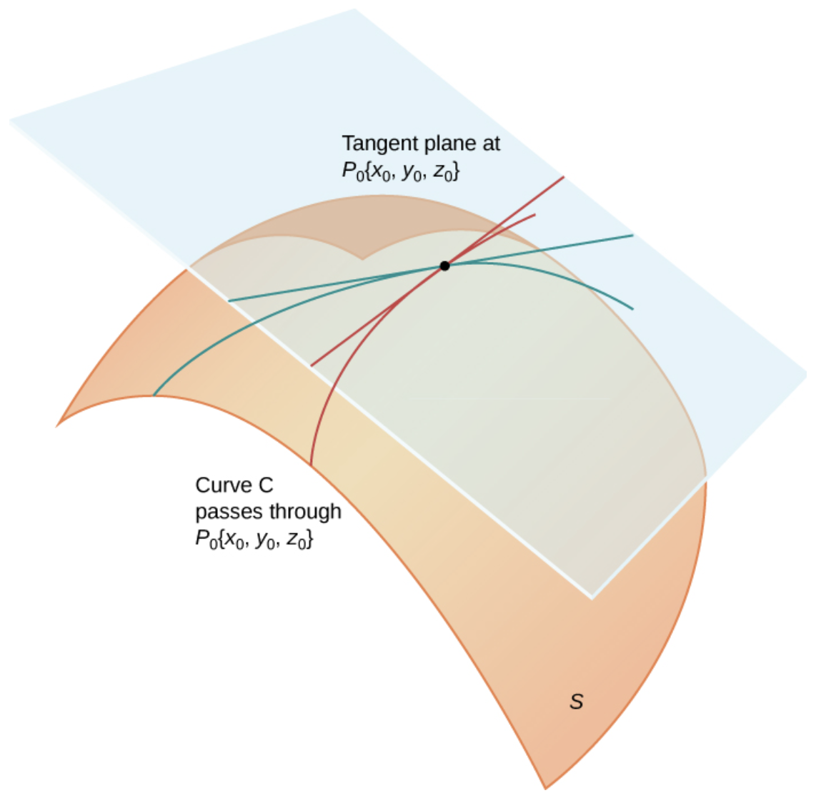
Let $S$ be a surface, and $\mathbf{x}_0$ a point on $S\text{.}$ A tangent plane to $S$ at $\mathbf{x}_0$ is a plane that contains the tangent lines of any differentiable curve contained in $S$ as it passes through $\mathbf{x}_0\text{.}$

A tangent plane touching a surface along tangent lines through a point. — Figure 3.5.6. The tangent plane to a surface $S$ at a point $P_0$ contains all the tangent lines to curves in $S$ that pass through $P_0\text{.}$ Figure 4.27 from Edwin “Jed” Herman and Gilbert Strang, *Calculus Volume 3*, OpenStax, © 2018 Rice University, licensed under `CC BY-NC-SA 4.0`; source: `OpenStax Figure 4.27`.
🔗

🔗

Theorem 3.5.7. Equation of the Tangent Plane.

Suppose $S$ is the graph of a function $f(x,y)$ which is differentiable at a point $(x_0,y_0)\text{.}$ Then the tangent plane to $S$ exists, is unique, and is described by the equation

\begin{equation*} z - f(x_0,y_0) = f_x(x_0,y_0) ( x - x_0 ) + f_y(x_0,y_0) (y - y_0)\text{.} \end{equation*}

Note that this plane is the graph of the linear approximation $L$ to $f$ at $(x_0,y_0)\text{.}$

🔗

Why is this true?.

We verify that the plane described by the equation above is the only possible tangent plane. Recall from Theorem 3.4.5 that the curve obtained by the intersection of $S$ with the plane $y = y_0$ has slope $f_x(x_0,y_0)$ at the point $(x_0,y_0)\text{,}$ and the tangent line to the curve at this point is by a line with direction vector $(1, 0, f_x(x_0,y_0))\text{.}$ Similarly, the curve obtained by the intersection of $S$ with the plane $x = x_0$ has slope $f_y(x_0,y_0)\text{,}$ and so the tangent line to the curve at this point is a line with direction vector $(0,1,f_y(x_0,y_0))\text{.}$ But now using the method of Activity 3.5.2, we see that a normal vector to the plane containing these two lines is of the form $\mathbf{n} = (-f_x(x_0,y_0),- f_y(x_0,y_0),1)\text{.}$ So the tangent plane to $S$ at $(x_0,y_0,f(x_0,y_0))$ must be described by the equation

\begin{equation*} (-f_x(x_0,y_0),- f_y(x_0,y_0),1) \cdot ( x - x_0, y - y_0, z - f(x_0,y_0) ) = 0\text{,} \end{equation*}

an equation we may rearrange to read

\begin{equation*} z - f(x_0,y_0) = f_x(x_0,y_0) ( x - x_0 ) + f_y(x_0,y_0) ( y - y_0 )\text{.} \end{equation*}

🔗

Activity 3.5.3.

Find an equation of the tangent plane to the surface

\begin{equation*} z = e^x\cos y \end{equation*}

at $(0,\frac{\pi}{2},0)\text{.}$

🔗

Solution.

The surface is the graph of the equation $f(x,y) = e^x \cos y\text{,}$ so we may use Theorem 3.5.7 to find the equation of the tangent plane. First, we calculate that

\begin{equation*} f(0,\pi/2) = e^0 \cos(\pi/2) = 0\text{.} \end{equation*}

Next, we calculate that

\begin{equation*} f_x(x,y) = e^x \cos y \quad\text{and}\quad f_y(x,y) = - e^x \sin y \end{equation*}

so $f_x(0,\pi/2) = e^0 \cos(\pi/2) = 0$ and $f_y(0,\pi/2) = - e^0 \sin(\pi/2) = -1\text{.}$ This means that an equation describing the tangent plane is given by

\begin{equation*} z - 0 = 0 (x - 0) + (-1) ( y - \pi/2 ) \end{equation*}

which simplifies to

\begin{equation*} z + y = \pi/2\text{.} \end{equation*}

🔗

Subsection Vector-valued local linearization

Subsubsection Linear maps reappear locally

A nonlinear map is usually not linear globally. Near one input, however, differentiability replaces small input changes by a linear map.

\begin{equation*} F(\mathbf{a}+\mathbf{h})\approx F(\mathbf{a})+J_F(\mathbf{a})\mathbf{h}. \end{equation*}

$\mathbf{x}\mapsto F(\mathbf{a})+J_F(\mathbf{a})(\mathbf{x}-\mathbf{a})$ is affine in $\mathbf{x}\text{.}$ $\mathbf{h}\mapsto J_F(\mathbf{a})\mathbf{h}$ is the linear map on input changes.

🔗

Linear algebra gave us global linear maps $\mathbf{x}\mapsto A\mathbf{x}\text{.}$ Calculus gives us local linear maps $\mathbf{h}\mapsto J_F(\mathbf{a})\mathbf{h}\text{.}$ The same matrix language therefore reappears inside nonlinear problems.

🔗

Definition 3.5.8. Linear Approximation of Vector-Valued Functions.

Let $F: \R^n \to \R^m$ be a vector-valued function. Provided that the partial derivatives of the components of $F$ all exist at $\mathbf{a}\text{,}$ so that the Jacobian matrix $J_F$ is well-defined, the linear approximation of $F$ at $\mathbf{a}$ is the vector-valued affine function

\begin{equation*} L(\mathbf{x}) = F(\mathbf{a}) + J_F(\mathbf{a})(\mathbf{x} - \mathbf{a}) \end{equation*}

where $J_F(\mathbf{a}) (\mathbf{x} - \mathbf{a})$ is the Jacobian matrix of $F$ evaluated at $\mathbf{a}\text{,}$ and then applied to the vector $\mathbf{x} - \mathbf{a}\text{.}$ The approximation is affine in $\mathbf{x}\text{;}$ its linear part is the map $\mathbf{h} \mapsto J_F(\mathbf{a})\mathbf{h}$ on small input changes.

🔗

The components of $L$ are precisely the linear approximations of the components of $F\text{,}$ i.e., $L_i(\mathbf{x}) = F_i(\mathbf{a}) + (\nabla F_i)(\mathbf{a})^T(\mathbf{x} - \mathbf{a})\text{.}$

🔗

Note 3.5.9.

Geometrically, the graph of the linear approximation to a vector-valued function can be visualized as a higher dimensional “tangent plane” of the graph of the function $F$ at $\mathbf{a}\text{.}$

🔗

Activity 3.5.4.

Let $F(x,y) = ( x^2y, xe^y )\text{.}$ Find the linear approximation of $F$ at the point $(1,0)\text{,}$ and use it to approximate $F(1.1, -0.2)\text{.}$

🔗

Solution.

We compute that

\begin{align*} J_F \amp = \begin{bmatrix} \frac{\partial}{\partial x} \{ x^2 y \} \amp \frac{\partial}{\partial y} \{ x^2 y \} \\ \frac{\partial}{\partial x} \{ xe^y \} \amp \frac{\partial}{\partial y} \{ xe^y \} \end{bmatrix}\\ \amp = \begin{bmatrix} 2xy \amp x^2 \\ e^y \amp xe^y \end{bmatrix}\text{.} \end{align*}

In particular,

\begin{equation*} J_F(1,0) = \begin{bmatrix} 2(1)(0) \amp (1)^2 \\ e^{(0)} \amp (1)e^{(0)} \end{bmatrix} = \begin{bmatrix} 0 \amp 1 \\ 1 \amp 1 \end{bmatrix}\text{.} \end{equation*}

Since

\begin{equation*} F(1,0) = \begin{bmatrix} (1)^2(0) \\ (1)e^{(0)} \end{bmatrix} = \begin{bmatrix} 0 \\ 1 \end{bmatrix}\text{.} \end{equation*}

So the linear approximation of $F$ at $(1,0)$ is the function

\begin{align*} L \begin{bmatrix} x \\ y \end{bmatrix} \amp = \begin{bmatrix} 0 \\ 1 \end{bmatrix} + \begin{bmatrix} 0 \amp 1 \\ 1 \amp 1 \end{bmatrix} \begin{bmatrix} x - 1 \\ y \end{bmatrix}\\ \amp = \begin{bmatrix} 1y \\ 1 + (x - 1) + y \end{bmatrix}\\ \amp = \begin{bmatrix} y \\ x + y \end{bmatrix}\text{.} \end{align*}

\begin{equation*} F(1.1,-0.2) \approx L(1.1,-0.2) = \begin{bmatrix} -0.2 \\ 1.1 - 0.2 \end{bmatrix} = \begin{bmatrix} -0.2 \\ 0.9 \end{bmatrix}\text{.} \end{equation*}

🔗

Activity 3.5.5. Local square-grid visualization.

Return to

\begin{equation*} F\left(\begin{bmatrix}x\\y\end{bmatrix}\right) = \begin{bmatrix} x+y^2\\ y \end{bmatrix}. \end{equation*}

🔗

The Jacobian matrix is

\begin{equation*} J_F(x,y) = \begin{bmatrix} 1&2y\\ 0&1 \end{bmatrix}. \end{equation*}

Let

\begin{equation*} \mathbf{a} = \begin{bmatrix} 0\\ 1/2 \end{bmatrix}. \end{equation*}

🔗

Compute $J_F(\mathbf{a})\text{.}$
🔗

🔗
Let $\mathbf{h}=\begin{bmatrix}h_1\\h_2\end{bmatrix}\text{.}$ Compute $F(\mathbf{a}+\mathbf{h})-F(\mathbf{a})\text{.}$
🔗

🔗
Compute $J_F(\mathbf{a})\mathbf{h}\text{.}$
🔗

🔗
Compute the error

\begin{equation*} F(\mathbf{a}+\mathbf{h})-F(\mathbf{a})-J_F(\mathbf{a})\mathbf{h}. \end{equation*}

🔗

🔗
If $0 \leq h_2 \leq r\text{,}$ how large can the first coordinate of the error be?
🔗

🔗
What happens to the local square-grid picture as $r$ gets smaller?
🔗

🔗

Solution.

Since $a_2=1/2\text{,}$

\begin{equation*} J_F(\mathbf{a}) = \begin{bmatrix} 1&1\\ 0&1 \end{bmatrix}. \end{equation*}

This is the horizontal shear matrix from Unit 1.

🔗

Now

\begin{equation*} \mathbf{a}+\mathbf{h} = \begin{bmatrix} h_1\\ 1/2+h_2 \end{bmatrix}. \end{equation*}

Thus

\begin{equation*} F(\mathbf{a}+\mathbf{h}) = \begin{bmatrix} h_1+(1/2+h_2)^2\\ 1/2+h_2 \end{bmatrix} = \begin{bmatrix} h_1+1/4+h_2+h_2^2\\ 1/2+h_2 \end{bmatrix}. \end{equation*}

Also,

\begin{equation*} F(\mathbf{a}) = \begin{bmatrix} 1/4\\ 1/2 \end{bmatrix}. \end{equation*}

🔗

Therefore

\begin{equation*} F(\mathbf{a}+\mathbf{h})-F(\mathbf{a}) = \begin{bmatrix} h_1+h_2+h_2^2\\ h_2 \end{bmatrix}. \end{equation*}

The Jacobian matrix prediction is

\begin{equation*} J_F(\mathbf{a})\mathbf{h} = \begin{bmatrix} 1&1\\ 0&1 \end{bmatrix} \begin{bmatrix} h_1\\ h_2 \end{bmatrix} = \begin{bmatrix} h_1+h_2\\ h_2 \end{bmatrix}. \end{equation*}

🔗

So the error is

\begin{equation*} F(\mathbf{a}+\mathbf{h})-F(\mathbf{a})-J_F(\mathbf{a})\mathbf{h} = \begin{bmatrix} h_2^2\\ 0 \end{bmatrix}. \end{equation*}

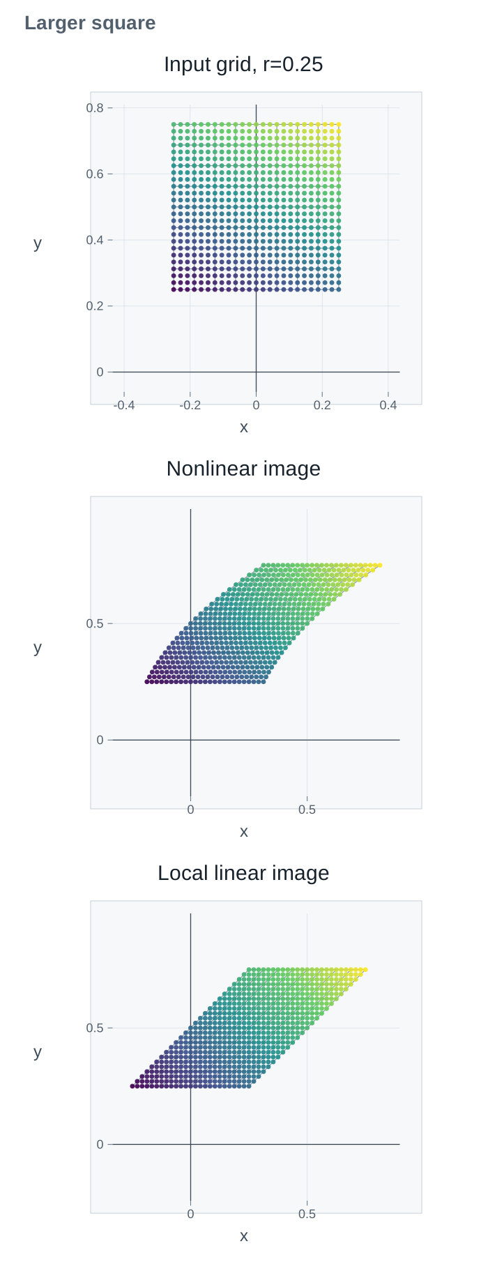
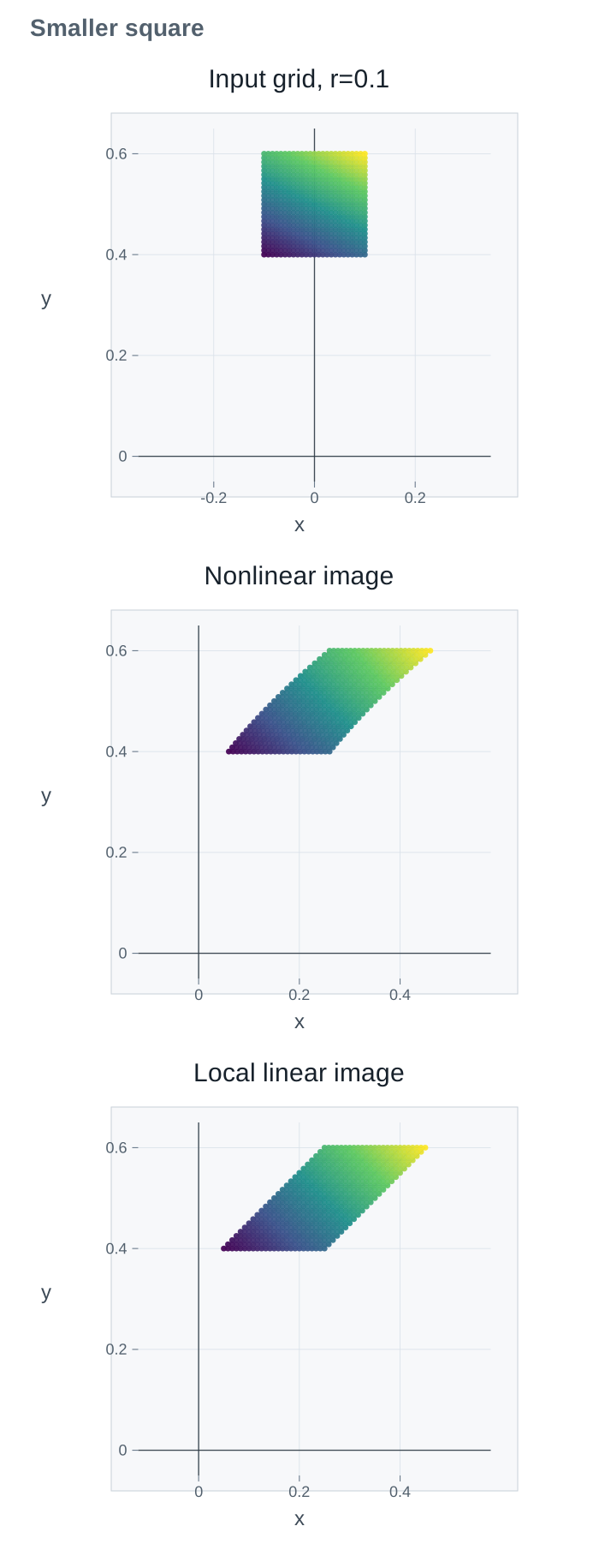
If $0 \leq h_2 \leq r\text{,}$ then $0 \leq h_2^2 \leq r^2\text{.}$ As the square around $\mathbf{a}$ shrinks, the nonlinear image and the local linear image become closer.

🔗

The local linear map acts on the change vector $\mathbf{h}\text{,}$ not on the original input vector $\mathbf{x}\text{.}$

🔗

Note 3.5.10.

The local square-grid visualization does not produce one matrix for the whole nonlinear map. It shows one matrix approximation near one base point.

🔗

Local square-grid comparison for the larger input square. — Figure 3.5.11. Local square-grid visualization near $\mathbf{a}=\begin{bmatrix}0\\1/2\end{bmatrix}$ for the larger input square $r=0.25\text{.}$ The three panels show the input grid, the nonlinear image, and the local linear image on ticked axes.
🔗

Local square-grid comparison for the smaller input square. — Figure 3.5.12. Local square-grid visualization near $\mathbf{a}=\begin{bmatrix}0\\1/2\end{bmatrix}$ for the smaller input square $r=0.1\text{.}$ The nonlinear image is closer to the local linear image than in the larger-square visualization.
🔗

🔗

Prev Top Next