MATH 345: Linear Algebra and Optimization

Section 1.1 Vectors

Subsection Vectors as lists of numbers

A real quantity is also called a scalar.

Definition 1.1.1. Vector.

An \(n\)-vector is an ordered list of \(n\) scalars, often written in the form \(\mathbf{v} = (v_1,v_2,\ldots,v_n)\text{.}\) The collection of all \(n\)-vectors is denoted \(\R^n\text{.}\)
We will also encounter vectors written as a row or column of numbers in square brackets, i.e.,
\begin{equation*} \begin{bmatrix} v_1 \amp \cdots \amp v_n \end{bmatrix} \quad\text{and}\quad \begin{bmatrix} v_1 \\ \vdots \\ v_n \end{bmatrix}\text{.} \end{equation*}
It is customary to use bold letters for variables, such as \(\mathbf{v}\) or \(\mathbf{w}\text{,}\) to represent vectors. We let \(\mathbf{0}\) denote the vector \((0,\dots,0)\) consisting only of zeros. A point in \(n\)-dimensional space can also be identified with an ordered list of \(n\) numbers using Cartesian coordinates. When referring specifically to a point \(P\text{,}\) we write \(P(x_1,x_2,\ldots,x_n)\) to indicate its coordinates.

Subsection Vectors as displacements in space

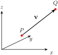
Vectors can be used to represent displacements between points in space. The vector \(\mathbf{v}=(v_1,v_2,v_3)\) represents the displacement from \(P(x_1,y_1,z_1)\) to \(Q(x_2,y_2,z_2)\text{,}\) where \(x_2 = x_1 + v_1\text{,}\) \(y_2 = y_1 + v_2\text{,}\) and \(z_2 = z_1 + v_3\text{.}\) This vector is also written as \(\overrightarrow{PQ}\text{.}\) Because vectors often indicate displacements, they are drawn pictorially as arrows starting at a point, and ending where that point is displaced by the vector.
A vector, represented as an arrow between two points.
Three coordinate axes labeled \(x\text{,}\) \(y\text{,}\) and \(z\) meet at an origin. A thick arrow labeled \(\mathbf{v}\) starts at the red point \(P\) and ends at the red point \(Q\text{,}\) showing the displacement from \(P\) to \(Q\text{.}\)
Figure 1.1.2. A vector \(\mathbf{v}\) represented as an arrow between two points \(P\) and \(Q\text{.}\)

Activity 1.1.1. Vectors as displacements in space.

What is the vector representing the displacement from the point \(P(1,2)\) to the point \(Q(5,7)\text{.}\)
Solution.
If \(\mathbf{v} = (v_1,v_2)\) was the displacement, then we would have \((1 + v_1, 2 + v_2) = (5,7)\text{,}\) i.e., so that \(1 + v_1 = 5\) and \(2 + v_2 = 7\text{.}\) Solving these equations gives \(v_1 = 4\) and \(v_2 = 5\text{,}\) so that the displacement vector is \(\mathbf{v} = (4,5)\text{.}\)

Definition 1.1.3. Length of a vector.

The length of a vector \(\mathbf{v} = (v_1,\dots,v_n)\) is the quantity
\begin{equation*} \| \mathbf{v} \| = \sqrt{ v_1^2 + \cdots + v_n^2 }\text{.} \end{equation*}

Activity 1.1.2.

Verify, using planar geometry, that the length of a \(2\)-vector is the length of the line-segment of the arrow representing the vector.
Solution.
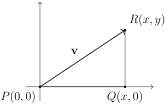
Let \(\mathbf{v} = (x,y)\) be an arbitrary \(2\)-vector. Consider a triangle with vertices \(P(0,0)\text{,}\) \(Q(x,0)\text{,}\) and \(R(x,y)\) (see FigureΒ 1.1.4).
A triangle drawn to determine the length of the line-segment upon which a 2-vector is based.
The figure shows \(x\)- and \(y\)-axes with a vector \(\mathbf{v}\) drawn from \(P(0,0)\) to \(R(x,y)\text{.}\) A horizontal segment from \(P\) to \(Q(x,0)\) and a vertical segment from \(Q\) to \(R\) form a right triangle whose hypotenuse is the vector.
Figure 1.1.4. A triangle with vertices \(P(0,0)\text{,}\) \(Q(x,0)\text{,}\) and \(R(x,y)\text{,}\) drawn to determine the length of the line-segment upon which a \(2\)-vector is based.
This triangle is right-angled (the two legs are horizontal and vertical), and the hypotenuse is the line-segment upon which the vector \(\mathbf{v}\) is built. The length of the leg from \(P(0,0)\) to \(Q(x,0)\) is \(|x|\text{,}\) and the length of the leg from \(Q(x,0)\) to \(R(x,y)\) is \(|y|\text{.}\) By Pythagoras’ theorem, we conclude that the length of the hypotenuse is
\begin{equation*} \sqrt{ |x|^2 + |y|^2 } = \sqrt{x^2 + y^2} = \| \mathbf{v} \|\text{.} \end{equation*}
In a calculus course, you may have mostly seen a vector as a displacement, but in this course it can also be a row of data or a list of model parameters, among other important applications. The same operations below will later compare documents, tokens, and feature vectors.

Subsection Adding and scaling vectors

Two displacements can be combined: just apply one displacement after the other is applied. This naturally leads to the notion of adding two vectors.

Definition 1.1.5. Adding vectors.

The sum of two \(n\)-vectors \(\mathbf{v} = (v_1,\dots,v_n)\) and \(\mathbf{w} = (w_1,\dots,w_n)\text{,}\) denoted \(\mathbf{v} + \mathbf{w}\text{,}\) is the vector given by the tuple \((v_1 + w_1, \dots, v_n + w_n)\text{.}\)

Remark 1.1.6.

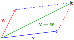
The sum of two vectors can be illustrated pictorially as in FigureΒ 1.1.7 by drawing the parallelogram with the vectors placed along two sides of the parallelogram.
The sum of two vectors.
A blue vector \(\mathbf{v}\) and a red vector \(\mathbf{w}\) start at the origin. Dashed copies of each vector are translated to the tip of the other vector, and both translated arrows meet at a shared endpoint. A green arrow from the origin to that endpoint is labeled \(\mathbf{v}+\mathbf{w}\text{.}\)
Figure 1.1.7. The sum of two vectors \(\mathbf{v}\) and \(\mathbf{w}\text{.}\)
One can also scale a vector by a given scalar quantity.

Definition 1.1.8. Scaling vectors.

If \(\mathbf{v} = (v_1,\cdots,v_n)\) is an \(n\)-vector and \(t \in \R\) is a scalar, we let \(t \mathbf{v}\) denote the vector \((tv_1, \cdots, tv_n)\text{,}\) i.e., multiplying each entry of the vector \(\mathbf{v}\) by \(t\text{.}\)

Definition 1.1.9. Linear combinations and convex combinations of vectors.

If \(\mathbf{v}_1,\ldots,\mathbf{v}_k\) are vectors in \(\mathbb R^n\) and \(c_1,\ldots,c_k\) are scalars, then
\begin{equation*} c_1\mathbf{v}_1+\cdots+c_k\mathbf{v}_k \end{equation*}
is a linear combination of \(\mathbf{v}_1,\ldots,\mathbf{v}_k\text{.}\) The scalars \(c_1,\ldots,c_k\) are the coefficients of the linear combination. If \(c_i\ge 0\) for all \(i\) and \(c_1+\cdots+c_k=1\text{,}\) then the linear combination is a convex combination.
A convex combination can be interpreted as a weighted average.

Activity 1.1.3. A weighted average.

Let \(\mathbf{v}_1=(10,0)\text{,}\) \(\mathbf{v}_2=(0,10)\text{,}\) \(\mathbf{v}_3=(10,10)\text{,}\) and \(\alpha=(1/4,1/4,1/2)\text{.}\) Compute \(\alpha_1\mathbf{v}_1+\alpha_2\mathbf{v}_2+\alpha_3\mathbf{v}_3\text{.}\)
Solution.
We have
\begin{equation*} \frac14(10,0)+\frac14(0,10)+\frac12(10,10)=(7.5,7.5). \end{equation*}
The coefficients are nonnegative and add to \(1\text{,}\) so this is a convex combination.

Subsection Dot products of vectors

Definition 1.1.10. Dot product.

The dot product of two \(n\)-vectors \(\mathbf{v} = (v_1,\dots,v_n)\) and \(\mathbf{w} = (w_1,\dots,w_n)\) is the scalar quantity
\begin{equation*} \mathbf{v} \cdot \mathbf{w} = v_1 w_1 + \cdots + v_n w_n\text{.} \end{equation*}
Geometrically, the dot product of two vectors is a quantity which is related to the angle between the two vectors \(\mathbf{v}\) and \(\mathbf{w}\text{.}\) If we draw the two vectors as arrows with the same starting point, then they form an angle on the plane containing both vectors, and the angle \(\theta\) is given below.
The dot product can be thought of as a measure of the similarity between two vectors. Suppose \(\theta\) is the angle between two vectors \(\mathbf{v}\) and \(\mathbf{w}\text{:}\)
  • If \(\theta\) is close to zero, then the two vectors are close to pointing in the same direction. Since \(\cos(0^\circ) = 1\text{,}\) this occurs precisely when
    \begin{equation*} \frac{\mathbf{v} \cdot \mathbf{w}}{\| \mathbf{v} \| \| \mathbf{w} \|} \approx 1\text{.} \end{equation*}
  • If \(\theta\) is close to \(180^\circ\text{,}\) then the two vectors are close to pointing in opposite directions. Since \(\cos(180^\circ) = -1\text{,}\) this occurs precisely when
    \begin{equation*} \frac{\mathbf{v} \cdot \mathbf{w}}{\| \mathbf{v} \| \| \mathbf{w} \|} \approx -1\text{.} \end{equation*}
  • If \(\theta\) is close to \(90^\circ\text{,}\) the two vectors are close to pointing at right angles. Since \(\cos(90^\circ) = 0\text{,}\) this occurs precisely when
    \begin{equation*} \frac{\mathbf{v} \cdot \mathbf{w}}{\| \mathbf{v} \| \| \mathbf{w} \|} \approx 0\text{.} \end{equation*}
    When \(\mathbf{v} \cdot \mathbf{w} = 0\text{,}\) so that \(\theta = 90^\circ\text{,}\) we say the two vectors are perpendicular, or orthogonal.
Thus the quantity
\begin{equation*} \frac{\mathbf{v} \cdot \mathbf{w}}{\| \mathbf{v} \| \| \mathbf{w} \|} \end{equation*}
ranges between \(-1\) and \(1\text{,}\) and measures the degree to which the two vectors \(\mathbf{v}\) and \(\mathbf{w}\) point in the same, or opposite, directions. In some contexts, especially in certain areas of data science, this quantity is called the cosine similarity between the vectors \(\mathbf{v}\) and \(\mathbf{w}\text{.}\)

Warning 1.1.12.

Cosine similarity is undefined if either vector is the zero vector.

Activity 1.1.4.

Calculate the angle between the two vectors \(\mathbf{v} = (1,2)\) and \(\mathbf{w} = (\sqrt{3} + 2, 2\sqrt{3} - 1)\text{.}\)
Solution.
We begin by calculating the lengths of the two vectors, i.e
\begin{equation*} \| \mathbf{v} \| = \sqrt{ (1)^2 + (2)^2 } = \sqrt{5} \end{equation*}
and
\begin{align*} \| \mathbf{w} \| \amp = \sqrt{ (\sqrt{3} + 2)^2 + (2\sqrt{3} - 1)^2 }\\ \amp = \sqrt{ (3 + 4 \sqrt{3} + 4) + (12 - 4 \sqrt{3} + 1) }\\ \amp = \sqrt{20}\text{.} \end{align*}
Next, we calculate the dot product
\begin{align*} \mathbf{v} \cdot \mathbf{w} \amp = (1)(\sqrt{3} + 2) + (2)(2\sqrt{3} - 1)\\ \amp = \sqrt{3} + 2 + 4\sqrt{3} - 2\\ \amp = 5 \sqrt{3}\text{.} \end{align*}
If \(\theta\) is the angle between the two vectors, then
\begin{align*} \cos(\theta) \amp = \frac{\mathbf{v} \cdot \mathbf{w}}{\| \mathbf{v} \| \| \mathbf{w} \|}\\ \amp = \frac{5 \sqrt{3}}{\sqrt{5} \sqrt{20}}\\ \amp = \sqrt{3}/2\text{.} \end{align*}
Thus the angle between the two vectors is
\begin{equation*} \theta = \cos^{-1}( \sqrt{3}/2 ) = 30^\circ\text{.} \end{equation*}
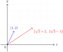
The two vectors from ActivityΒ 1.1.4.
A dashed coordinate grid is shown with \(x\)- and \(y\)-axes. A blue arrow from the origin ends at \((1,2)\text{,}\) while a longer red arrow from the origin ends at \((\sqrt{3}+2, 2\sqrt{3}-1)\text{.}\) The two arrows form the angle used in the dot-product activity.
Figure 1.1.13. The vectors \(\mathbf{v}\) and \(\mathbf{w}\) from ActivityΒ 1.1.4, drawn as arrows from the origin.

Activity 1.1.5.

Calculate the angle between the two vectors
\begin{equation*} \mathbf{v} = \begin{bmatrix} 2 \\ 3 \\ 0 \\ 2 \end{bmatrix} \quad\text{and}\quad \mathbf{w} = \begin{bmatrix} 1 \\ 0 \\ 1 \\ -1 \end{bmatrix}\text{.} \end{equation*}
Solution.
We calculate that
\begin{equation*} \mathbf{v} \cdot \mathbf{w} = (2)(1) + (3)(0) + (0)(1) + (2)(-1) = 2 + 0 + 0 - 2 = 0\text{.} \end{equation*}
Thus if \(\theta\) is the angle between the two vectors, then
\begin{equation*} \cos(\theta) = \frac{\mathbf{v} \cdot \mathbf{w}}{\| \mathbf{v} \| \| \mathbf{w} \|} = \frac{0}{\| \mathbf{v} \| \| \mathbf{w} \|} = 0\text{.} \end{equation*}
Thus
\begin{equation*} \theta = \cos^{-1}(0) = 90^\circ\text{.} \end{equation*}

Note 1.1.14.

Note that \(\| \mathbf{v} \|^2 = \mathbf{v} \cdot \mathbf{v}\) for any \(\mathbf{v} \in \R^n\text{.}\)
We will study the dot product in far more detail in UnitΒ 4 and UnitΒ 7.

Definition 1.1.15. Distance between vectors.

The Euclidean distance between two vectors \(\mathbf{u},\mathbf{v} \in \R^n\) is
\begin{equation*} \operatorname{dist}(\mathbf{u},\mathbf{v}) = \| \mathbf{u} - \mathbf{v} \|. \end{equation*}
It measures how far apart the endpoints are, while cosine similarity compares direction after normalization.

Subsection Applications of vectors

Vectors can represent quantities other than displacements. The entries of a vector can record measurements, counts, samples, or features. The meaning of a vector depends on what its coordinates represent.
Table 1.1.16. Some vector representations
Object Meaning of the entries
Color red, green, and blue intensities
Time series measurements at successive times
Portfolio amounts held in each asset
Image pixel intensities, listed in a fixed order
Document counts of selected words
Customer purchases of selected products
Object with features measured attributes such as size, price, weight, or rating
The same vector operations can have different interpretations. A sum can add purchases, add word counts, or add two time series. A scalar multiple can rescale an image, double a portfolio, or change units. A dot product can produce a score. A distance can compare two feature vectors. Cosine similarity compares direction after normalization.

Activity 1.1.6. Word-count vectors.

Use the dictionary linear, matrix, data. A document vector records the number of times these words appear, in this order. The query
\begin{equation*} \mathbf{q}=\begin{bmatrix}1\\0\\1\end{bmatrix} \end{equation*}
represents the phrase β€œlinear data”. Consider three document vectors
\begin{equation*} \mathbf{D}_1=\begin{bmatrix}2\\0\\2\end{bmatrix},\qquad \mathbf{D}_2=\begin{bmatrix}1\\1\\0\end{bmatrix},\qquad \mathbf{D}_3=\begin{bmatrix}0\\2\\0\end{bmatrix}. \end{equation*}
Compute the cosine similarities and Euclidean distances between \(\mathbf{q}\) and each \(\mathbf{D}_i\text{.}\) Rank the documents by cosine similarity.
Solution.
First,
\begin{align*} \operatorname{cosim}(\mathbf{q},\mathbf{D}_1) \amp= \frac{\mathbf{q}\cdot\mathbf{D}_1}{\|\mathbf{q}\|\|\mathbf{D}_1\|}\\ \amp= \frac{4}{\sqrt{2}\sqrt{8}}\\ \amp= 1. \end{align*}
Next,
\begin{align*} \operatorname{cosim}(\mathbf{q},\mathbf{D}_2) \amp= \frac{\mathbf{q}\cdot\mathbf{D}_2}{\|\mathbf{q}\|\|\mathbf{D}_2\|}\\ \amp= \frac{1}{\sqrt{2}\sqrt{2}}\\ \amp= \frac12. \end{align*}
Finally, \(\operatorname{cosim}(\mathbf{q},\mathbf{D}_3)=0\text{.}\) So the ranking by cosine similarity is
\begin{equation*} \mathbf{D}_1,\ \mathbf{D}_2,\ \mathbf{D}_3. \end{equation*}
For the Euclidean distances,
\begin{align*} \operatorname{dist}(\mathbf{q},\mathbf{D}_1) \amp= \|\mathbf{q}-\mathbf{D}_1\|\\ \amp= \left\|\begin{bmatrix}1\\0\\1\end{bmatrix}-\begin{bmatrix}2\\0\\2\end{bmatrix}\right\|\\ \amp= \left\|\begin{bmatrix}-1\\0\\-1\end{bmatrix}\right\|=\sqrt{2},\\ \operatorname{dist}(\mathbf{q},\mathbf{D}_2) \amp= \|\mathbf{q}-\mathbf{D}_2\|\\ \amp= \left\|\begin{bmatrix}1\\0\\1\end{bmatrix}-\begin{bmatrix}1\\1\\0\end{bmatrix}\right\|\\ \amp= \left\|\begin{bmatrix}0\\-1\\1\end{bmatrix}\right\|=\sqrt{2},\\ \operatorname{dist}(\mathbf{q},\mathbf{D}_3) \amp= \|\mathbf{q}-\mathbf{D}_3\|\\ \amp= \left\|\begin{bmatrix}1\\0\\1\end{bmatrix}-\begin{bmatrix}0\\2\\0\end{bmatrix}\right\|\\ \amp= \left\|\begin{bmatrix}1\\-2\\1\end{bmatrix}\right\|=\sqrt{6}. \end{align*}
The vector \(\mathbf{D}_1\) points in exactly the same direction as \(\mathbf{q}\) because \(\mathbf{D}_1=2\mathbf{q}\text{.}\) The vector \(\mathbf{D}_2\) shares the word β€œlinear” with the query but also contains β€œmatrix”. The vector \(\mathbf{D}_3\) contains only β€œmatrix”, so it is orthogonal to the query.
From the previous activity, we see that vectors can have high cosine similarity while being relatively far in terms of Euclidean distance.

Activity 1.1.7. The same ranking in code.

The following code repeats the cosine-similarity ranking from ActivityΒ 1.1.6.
import numpy as np

D1 = np.array([2, 0, 2], dtype=float)
D2 = np.array([1, 1, 0], dtype=float)
D3 = np.array([0, 2, 0], dtype=float)
q = np.array([1, 0, 1], dtype=float)

score1 = (D1 @ q) / (np.linalg.norm(D1) * np.linalg.norm(q))
score2 = (D2 @ q) / (np.linalg.norm(D2) * np.linalg.norm(q))
score3 = (D3 @ q) / (np.linalg.norm(D3) * np.linalg.norm(q))

score1, score2, score3
Output:
(1.0, 0.5, 0.0)
  1. Which score corresponds to \(\mathbf{D}_2\text{?}\)
  2. Where does the code compute \(\mathbf{D}_1\cdot\mathbf{q}\text{?}\)
  3. Which document is most similar to the query by cosine similarity?
  4. Why does the output agree with the word-count vector activity?
Solution.
The score for \(\mathbf{D}_2\) is score2. The expression D1 @ q computes \(\mathbf{D}_1\cdot\mathbf{q}\text{.}\) Since score1 is largest, \(\mathbf{D}_1\) is most similar to the query. The output agrees with the hand calculation: \(1,\frac12,0\text{.}\)

Example 1.1.17. Neural networks and transformers.

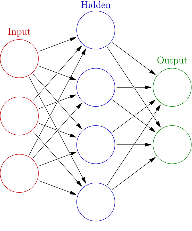
A neural network is a function built from layers. A layer takes numbers as input, combines them using weights, applies a rule, and sends output numbers to the next layer. In many neural networks, the input and output of a layer are vectors. The weights are adjusted from data during training.
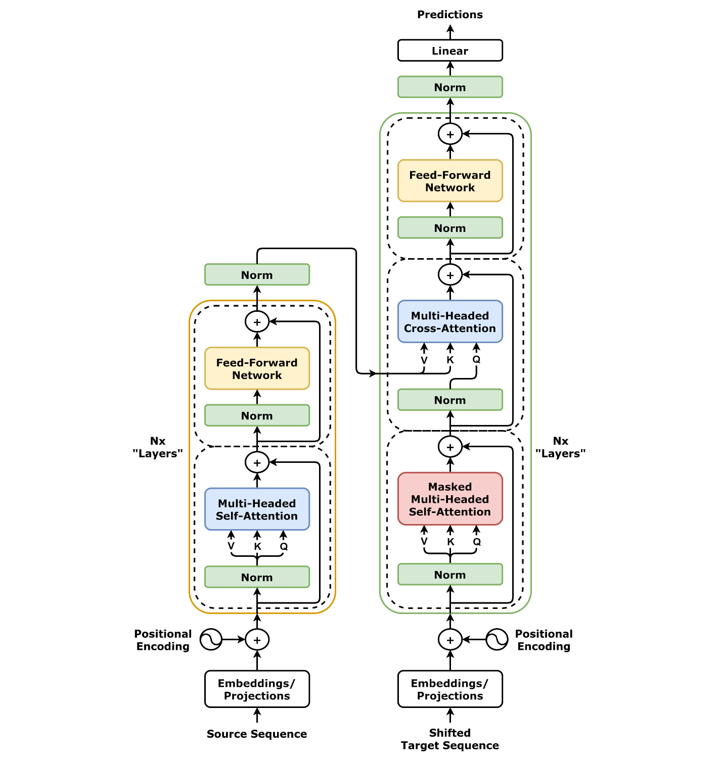
A transformer is a neural-network architecture for sequences. In a language model, text is first broken into tokens. A token can be a word, part of a word, punctuation mark, or other text fragment. Each token is represented by a vector.
A neural network diagram with input, hidden, and output layers.
Three red input nodes are arranged vertically on the left, four blue hidden-layer nodes appear in the center, and two green output nodes appear on the right. Black arrows connect each input node to the hidden layer, and gray arrows connect the hidden layer to the outputs, showing information moving left to right through the network.
Figure 1.1.18. A neural network diagram with input, hidden, and output layers. Source: Wikipedia, Neural network (machine learning), using Colored neural network.svg by Glosser.ca, derivative of Artificial neural network.svg, licensed under CC BY-SA 3.0.
A transformer processes a sequence of token vectors.
The diagram has two vertical stacks: an encoder stack for a source sequence on the left and a decoder stack for a target sequence on the right. Each stack shows embeddings and positional encoding feeding into attention and feed-forward blocks, with arrows indicating repeated layers. The decoder also points upward to a final linear and softmax prediction step.
Figure 1.1.19. A transformer processes a sequence of token vectors. The activities below focus on the vector operations visible in the diagram: token embeddings, dot-product scores, weighted averages, and affine layers. Source: Wikipedia, Transformer (deep learning architecture), using Transformer, full architecture.png by dvgodoy, licensed under CC BY 4.0.

Activity 1.1.8. A tiny attention-style token-weighting calculation.

Consider the token sequence
\begin{equation*} \text{small}, \qquad \text{red}, \qquad \text{bird}. \end{equation*}
Suppose a transformer layer is updating the token β€œbird”. Its query vector represents what this token is looking for in the sequence. Each key vector represents how another token can be matched by a query. Each value vector is the vector that may be averaged into the updated representation.
For this activity, the score for token \(i\) is
\begin{equation*} \operatorname{score}_i=\mathbf{q}_{\text{bird}}\cdot \mathbf{k}_i. \end{equation*}
Use
\begin{equation*} \mathbf{q}_{\text{bird}}=\begin{bmatrix}1\\1\end{bmatrix},\qquad \mathbf{k}_{\text{small}}=\begin{bmatrix}1\\0\end{bmatrix},\qquad \mathbf{k}_{\text{red}}=\begin{bmatrix}0\\1\end{bmatrix},\qquad \mathbf{k}_{\text{bird}}=\begin{bmatrix}1\\1\end{bmatrix}. \end{equation*}
  1. Compute the three scores
    \begin{equation*} \mathbf{q}_{\text{bird}}\cdot \mathbf{k}_{\text{small}},\qquad \mathbf{q}_{\text{bird}}\cdot \mathbf{k}_{\text{red}},\qquad \mathbf{q}_{\text{bird}}\cdot \mathbf{k}_{\text{bird}}. \end{equation*}
  2. Normalize the positive scores by dividing each score by the sum of all three scores. Call the resulting weights
    \begin{equation*} \boldsymbol{\alpha}= \begin{bmatrix} \alpha_{\text{small}}\\ \alpha_{\text{red}}\\ \alpha_{\text{bird}} \end{bmatrix}. \end{equation*}
  3. Use the value vectors
    \begin{equation*} \mathbf{v}_{\text{small}}=\begin{bmatrix}4\\0\end{bmatrix},\qquad \mathbf{v}_{\text{red}}=\begin{bmatrix}0\\4\end{bmatrix},\qquad \mathbf{v}_{\text{bird}}=\begin{bmatrix}4\\4\end{bmatrix} \end{equation*}
    to compute
    \begin{equation*} \mathbf{h}_{\text{bird}} = \alpha_{\text{small}}\mathbf{v}_{\text{small}} + \alpha_{\text{red}}\mathbf{v}_{\text{red}} + \alpha_{\text{bird}}\mathbf{v}_{\text{bird}}. \end{equation*}
  4. Which token receives the largest weight? Why?
Solution.
The scores are
\begin{equation*} \mathbf{q}_{\text{bird}}\cdot \mathbf{k}_{\text{small}}=1,\qquad \mathbf{q}_{\text{bird}}\cdot \mathbf{k}_{\text{red}}=1,\qquad \mathbf{q}_{\text{bird}}\cdot \mathbf{k}_{\text{bird}}=2. \end{equation*}
The sum of the scores is
\begin{equation*} 1+1+2=4. \end{equation*}
Thus
\begin{equation*} \boldsymbol{\alpha} = \begin{bmatrix} 1/4\\ 1/4\\ 1/2 \end{bmatrix}. \end{equation*}
The weighted average is
\begin{equation*} \mathbf{h}_{\text{bird}} = \frac14 \begin{bmatrix}4\\0\end{bmatrix} + \frac14 \begin{bmatrix}0\\4\end{bmatrix} + \frac12 \begin{bmatrix}4\\4\end{bmatrix} = \begin{bmatrix}3\\3\end{bmatrix}. \end{equation*}
The token β€œbird” receives the largest weight because its key vector has the largest dot product with \(\mathbf{q}_{\text{bird}}\text{.}\) The updated vector is a weighted average of the value vectors.

Warning 1.1.20.

This toy calculation uses normalization by the sum of positive scores to keep the arithmetic simple. Real transformer attention usually uses a different weighting rule.