Contents
Dark Mode Prev Up Next
\(\newcommand{\N}{\mathbb{N}}
\newcommand{\Z}{\mathbb{Z}}
\newcommand{\Q}{\mathbb{Q}}
\newcommand{\R}{\mathbb{R}}
\newcommand{\dimens}{\operatorname{dim}}
\DeclareMathOperator{\row}{\operatorname{row}}
\DeclareMathOperator{\col}{\operatorname{col}}
\newcommand{\im}{\operatorname{im}}
\newcommand{\nulls}{\operatorname{null}}
\newcommand{\minor}{\operatorname{minor}}
\newcommand{\spans}{\operatorname{span}}
\newcommand{\nullity}{\operatorname{nullity}}
\newcommand{\kers}{\operatorname{ker}}
\newcommand{\proj}{\operatorname{proj}}
\newcommand{\diag}{\operatorname{diag}}
\newcommand{\Tr}{\operatorname{Tr}}
\newcommand{\rank}{\operatorname{rank}}
\newcommand{\lt}{<}
\newcommand{\gt}{>}
\newcommand{\amp}{&}
\definecolor{fillinmathshade}{gray}{0.9}
\newcommand{\fillinmath}[1]{\mathchoice{\colorbox{fillinmathshade}{$\displaystyle \phantom{\,#1\,}$}}{\colorbox{fillinmathshade}{$\textstyle \phantom{\,#1\,}$}}{\colorbox{fillinmathshade}{$\scriptstyle \phantom{\,#1\,}$}}{\colorbox{fillinmathshade}{$\scriptscriptstyle\phantom{\,#1\,}$}}}
\)
Section 6.4 Singular value decomposition
The previous section found singular values from
\(A^TA\text{.}\) This section packages the same information into one factorization. The right singular vectors are special input directions. The singular values are stretch factors. The left singular vectors are the corresponding output directions.
The singular value decomposition is the rectangular analogue of orthogonal diagonalization. Orthogonal diagonalization applies to symmetric square matrices. SVD applies to every real matrix.
Definition 6.4.1 . Singular value decomposition.
Let \(A\) be an \(m\times n\) matrix, and let \(s=\min(m,n)\text{.}\) A singular value decomposition, or SVD, of \(A\) is a factorization
\begin{equation*}
A=U\Sigma V^T,
\end{equation*}
where \(U\) is an \(m\times m\) orthogonal matrix, \(V\) is an \(n\times n\) orthogonal matrix, and \(\Sigma\) is an \(m\times n\) diagonal matrix whose diagonal entries
\begin{equation*}
\sigma_1\geq \sigma_2\geq \cdots \geq \sigma_s\geq 0
\end{equation*}
are nonnegative.
The numbers \(\sigma_i\) are the singular values of \(A\text{.}\) The columns
\begin{equation*}
\mathbf{u}_1,\ldots,\mathbf{u}_m
\end{equation*}
of \(U\) are left singular vectors. The columns
\begin{equation*}
\mathbf{v}_1,\ldots,\mathbf{v}_n
\end{equation*}
of \(V\) are right singular vectors.
If \(r\) is the number of positive singular values, then
\begin{equation*}
A\mathbf{v}_i=\sigma_i\mathbf{u}_i
\qquad
\text{for }1\leq i\leq r,
\end{equation*}
and
\begin{equation*}
A\mathbf{v}_i=\mathbf{0}
\qquad
\text{for }i>r.
\end{equation*}
The factorization also gives a coordinate formula. If \(r=\operatorname{rank}(A)\text{,}\) then
\begin{equation*}
A\mathbf{x}
=
\sum_{i=1}^r
\sigma_i(\mathbf{v}_i\cdot\mathbf{x})\mathbf{u}_i.
\end{equation*}
The dot product \(\mathbf{v}_i\cdot\mathbf{x}\) measures how much of the input points in the \(i\) -th right singular direction. The singular value \(\sigma_i\) stretches that coordinate. The vector \(\mathbf{u}_i\) gives the output direction.
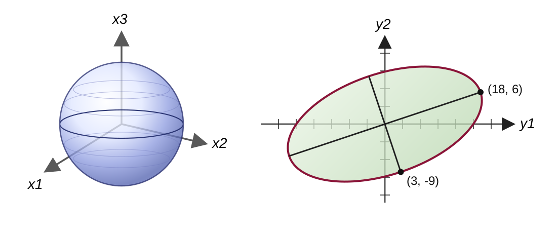
An
\(m \times n\) matrix
\(A\) maps the unit sphere (the set of all unit vectors) in
\(\R^n\) to an ellipsoid in
\(\mathbb{R}^m\) (i.e., a sphere which has been stretched and compressed along different
principal axes ). The singular value decomposition identifies the principal axes of this ellipsoid and the corresponding scaling factors.
FigureΒ 6.4.3 gives an example of how this may be visualized when
\(A\) is a
\(2 \times 3\) matrix.
The left side shows a blue unit sphere with coordinate axes labeled
\(x_1\text{,}\) \(x_2\text{,}\) and
\(x_3\text{.}\) The right side shows a green ellipse in a two-dimensional coordinate plane with axes labeled
\(y_1\) and
\(y_2\text{.}\) Two black line segments mark the principal semiaxes of the ellipse, ending at
\((18,6)\) and
\((3,-9)\text{.}\)
Figure 6.4.3. A matrix map from \(\mathbb{R}^3\) to \(\mathbb{R}^2\) corresponding to the matrix
\begin{equation*}
A = \begin{bmatrix} 4 \amp 11 \amp 14 \\ 8 \amp 7 \amp -2 \end{bmatrix}\text{.}
\end{equation*}
The left panel shows the unit sphere in \(\mathbb{R}^3\text{.}\) The right panel shows its image under \(A\) in \(\mathbb{R}^2\text{,}\) an ellipse with principal semiaxis endpoints \((18,6)\) and \((3,-9)\text{.}\) Adapted from David C. Lay, Steven R. Lay, and Judi J. McDonald, Linear Algebra and Its Applications , 6th edition, Pearson, Β© 2021, Pearson .
Lemma 6.4.4 . Properties of \(A^TA\) and \(AA^T\) .
Let \(A\) be an \(m\times n\) matrix. Then:
The eigenvalues of
\(A^TA\) and
\(AA^T\) are real and non-negative.
\(A^TA\) and
\(AA^T\) have the same set of positive eigenvalues.
Why is this true?.
1. The matrices
\(A^T A\) and
\(A A^T\) are symmetric, so by
TheoremΒ 5.4.8 their eigenvalues are real. If
\(A^T A \mathbf{v} = \lambda \mathbf{v}\) for
\(\mathbf{v} \neq \mathbf{0}\text{,}\) we calculate that
\begin{align*}
\|A\mathbf{v}\|^2 \amp = (A\mathbf{v})^T(A\mathbf{v}) = \mathbf{v}^TA^TA\mathbf{v} = \mathbf{v}^T\lambda\mathbf{v} = \lambda\|\mathbf{v}\|^2
\end{align*}
Since \(\|A\mathbf{v}\|^2 \geq 0\) and \(\|\mathbf{v}\|^2 > 0\text{,}\) we conclude that \(\lambda \geq 0\text{.}\)
2. Let \(\lambda\) be a positive eigenvalue of \(A^TA\) with eigenvector \(\mathbf{v} \neq \mathbf{0}\text{.}\) Then \(A^TA\mathbf{v} = \lambda\mathbf{v}\text{.}\) Let \(\mathbf{w} = A\mathbf{v}\text{.}\) Note that \(\mathbf{w} \neq \mathbf{0}\) since \(\lambda > 0\text{.}\) We have:
\begin{align*}
AA^T\mathbf{w} \amp = AA^T(A\mathbf{v}) = A(A^TA\mathbf{v}) = A(\lambda\mathbf{v}) = \lambda\mathbf{w}.
\end{align*}
So \(\lambda\) is also an eigenvalue of \(AA^T\text{.}\) The argument works in reverse by replacing \(A\) with \(A^T\text{,}\) proving that \(A^TA\) and \(AA^T\) have the same positive eigenvalues.
Theorem 6.4.5 . Computing the Singular Value Decomposition.
Given an \(m\times n\) matrix \(A\text{,}\) one way to obtain an SVD
\begin{equation*}
A=U\Sigma V^T
\end{equation*}
is as follows.
Find an orthonormal eigenbasis
\begin{equation*}
\mathbf{v}_1,\ldots,\mathbf{v}_n
\end{equation*}
for \(A^TA\text{.}\) Let \(\lambda_i\) be the eigenvalue associated with \(\mathbf{v}_i\text{.}\) Order the vectors so that
\begin{equation*}
\lambda_1\geq\lambda_2\geq\cdots\geq\lambda_r>0
\end{equation*}
and \(\lambda_i=0\) for \(i>r\text{.}\)
Define
\begin{equation*}
\sigma_i=\sqrt{\lambda_i}.
\end{equation*}
For \(1\leq i\leq r\text{,}\) define
\begin{equation*}
\mathbf{u}_i=\frac{1}{\sigma_i}A\mathbf{v}_i.
\end{equation*}
Extend
\begin{equation*}
\mathbf{u}_1,\ldots,\mathbf{u}_r
\end{equation*}
to an orthonormal basis
\begin{equation*}
\mathbf{u}_1,\ldots,\mathbf{u}_m
\end{equation*}
of \(\mathbb R^m\text{.}\)
Set
\begin{equation*}
V=[\mathbf{v}_1\ \cdots\ \mathbf{v}_n],
\qquad
U=[\mathbf{u}_1\ \cdots\ \mathbf{u}_m],
\end{equation*}
and let \(\Sigma\) be the \(m\times n\) diagonal matrix with diagonal entries \(\sigma_1,\ldots,\sigma_r\) followed by zeros.
Then
\begin{equation*}
A=U\Sigma V^T.
\end{equation*}
Why is this true?.
For \(i\neq j\) with \(1\leq i,j\leq r\text{,}\)
\begin{align*}
\mathbf{u}_i\cdot\mathbf{u}_j\\
\amp = \frac{1}{\sigma_i\sigma_j}(A\mathbf{v}_i)\cdot(A\mathbf{v}_j)\\
\amp = \frac{1}{\sigma_i\sigma_j}\mathbf{v}_i^T A^TA\mathbf{v}_j.\text{.}
\end{align*}
Since \(A^TA\mathbf{v}_j=\lambda_j\mathbf{v}_j\text{,}\) this becomes
\begin{equation*}
\frac{\lambda_j}{\sigma_i\sigma_j}
(\mathbf{v}_i\cdot\mathbf{v}_j)=0.
\end{equation*}
Also,
\begin{align*}
\|\mathbf{u}_i\|^2\\
\amp = \frac{1}{\sigma_i^2}\|A\mathbf{v}_i\|^2\\
\amp = \frac{1}{\lambda_i}\mathbf{v}_i^TA^TA\mathbf{v}_i\\
\amp = 1.
\end{align*}
Thus \(\mathbf{u}_1,\ldots,\mathbf{u}_r\) are orthonormal.
If \(i>r\text{,}\) then \(\lambda_i=0\text{,}\) so
\begin{align*}
\|A\mathbf{v}_i\|^2\\
\amp = \mathbf{v}_i^TA^TA\mathbf{v}_i\\
\amp = 0.
\end{align*}
Therefore \(A\mathbf{v}_i=\mathbf{0}\text{.}\)
Now compare the columns of \(AV\) and \(U\Sigma\text{:}\)
\begin{align*}
AV\\
\amp = [A\mathbf{v}_1\ \cdots\ A\mathbf{v}_n]\\
\amp = [\sigma_1\mathbf{u}_1\ \cdots\ \sigma_r\mathbf{u}_r\ \mathbf{0}\ \cdots\ \mathbf{0}]\\
\amp = U\Sigma.
\end{align*}
Since \(V\) is orthogonal, \(V^{-1}=V^T\text{.}\) Multiplying \(AV=U\Sigma\) on the right by \(V^T\) gives
\begin{equation*}
A=U\Sigma V^T.
\end{equation*}
The same computation also shows that the image of \(A\) is spanned by
\begin{equation*}
\mathbf{u}_1,\ldots,\mathbf{u}_r,
\end{equation*}
so \(r=\operatorname{rank}(A)\text{.}\)
Here is one complete SVD computation, broken into the same steps as the theorem.
Activity 6.4.1 . Computing an SVD, part 1: right singular vectors.
Let
\begin{equation*}
A = \begin{bmatrix} 1 \amp -1 \\ -2 \amp 2 \\ 2 \amp -2 \end{bmatrix}\text{.}
\end{equation*}
Find the eigenvalues of
\(A^TA\text{.}\)
Find an orthonormal eigenbasis
\begin{equation*}
\mathbf{v}_1,\mathbf{v}_2
\end{equation*}
for \(A^TA\text{,}\) with the positive eigenvalue first.
Find the singular values of
\(A\text{.}\)
Solution .
We compute
\begin{align*}
A^TA\\
\amp =
\begin{bmatrix}
1 \amp -2 \amp 2\\
-1 \amp 2 \amp -2
\end{bmatrix}
\begin{bmatrix}
1 \amp -1\\
-2 \amp 2\\
2 \amp -2
\end{bmatrix}\\
\amp =
\begin{bmatrix}
9 \amp -9\\
-9 \amp 9
\end{bmatrix}.
\end{align*}
The characteristic polynomial is
\begin{align*}
\det(A^TA-\lambda I)\\
\amp =
\det
\begin{bmatrix}
9-\lambda \amp -9\\
-9 \amp 9-\lambda
\end{bmatrix}\\
\amp = \lambda(\lambda-18).
\end{align*}
Thus the eigenvalues are
\begin{equation*}
\lambda_1=18,
\qquad
\lambda_2=0.
\end{equation*}
For \(\lambda_1=18\text{,}\) one eigenvector is
\begin{equation*}
\begin{bmatrix}
1\\
-1
\end{bmatrix},
\end{equation*}
so we choose the unit vector
\begin{equation*}
\mathbf{v}_1=
\frac{1}{\sqrt2}
\begin{bmatrix}
1\\
-1
\end{bmatrix}.
\end{equation*}
For \(\lambda_2=0\text{,}\) one eigenvector is
\begin{equation*}
\begin{bmatrix}
1\\
1
\end{bmatrix},
\end{equation*}
so we choose
\begin{equation*}
\mathbf{v}_2=
\frac{1}{\sqrt2}
\begin{bmatrix}
1\\
1
\end{bmatrix}.
\end{equation*}
The singular values are the square roots of the eigenvalues of \(A^TA\text{:}\)
\begin{equation*}
\sigma_1=\sqrt{18}=3\sqrt2,
\qquad
\sigma_2=0.
\end{equation*}
Activity 6.4.2 . Computing an SVD, part 2: output directions.
Use the vectors from the previous activity.
Compute
\(A\mathbf{v}_1\text{.}\)
Compute
\(A\mathbf{v}_2\text{.}\)
Compute
\begin{equation*}
\mathbf{u}_1=\frac{1}{\sigma_1}A\mathbf{v}_1.
\end{equation*}
What does
\(A\mathbf{v}_2=\mathbf{0}\) say about the matrix map?
Solution .
First,
\begin{align*}
A\mathbf{v}_1\\
\amp =
\begin{bmatrix}
1 \amp -1\\
-2 \amp 2\\
2 \amp -2
\end{bmatrix}
\frac{1}{\sqrt2}
\begin{bmatrix}
1\\
-1
\end{bmatrix}\\
\amp =
\begin{bmatrix}
\sqrt2\\
-2\sqrt2\\
2\sqrt2
\end{bmatrix}.
\end{align*}
Since \(\sigma_1=3\sqrt2\text{,}\)
\begin{align*}
\mathbf{u}_1\\
\amp =
\frac{1}{3\sqrt2}
\begin{bmatrix}
\sqrt2\\
-2\sqrt2\\
2\sqrt2
\end{bmatrix}\\
\amp =
\begin{bmatrix}
1/3\\
-2/3\\
2/3
\end{bmatrix}.
\end{align*}
Also,
\begin{align*}
A\mathbf{v}_2\\
\amp =
\begin{bmatrix}
1 \amp -1\\
-2 \amp 2\\
2 \amp -2
\end{bmatrix}
\frac{1}{\sqrt2}
\begin{bmatrix}
1\\
1
\end{bmatrix}\\
\amp =
\begin{bmatrix}
0\\
0\\
0
\end{bmatrix}.
\end{align*}
Thus
\(\mathbf{v}_2\) is a right null direction. The matrix map forgets that input direction. Since only one singular value is positive, the rank of
\(A\) is
\(1\text{.}\)
Activity 6.4.3 . Computing an SVD, part 3: assembling the factorization.
The SVD computation needs an orthonormal basis of \(\mathbb R^3\) beginning with
\begin{equation*}
\mathbf{u}_1=
\begin{bmatrix}
1/3\\
-2/3\\
2/3
\end{bmatrix}.
\end{equation*}
Use the following completion:
\begin{equation*}
\mathbf{u}_2=
\begin{bmatrix}
(2/3)\sqrt2\\
(1/6)\sqrt2\\
-(1/6)\sqrt2
\end{bmatrix},
\qquad
\mathbf{u}_3=
\begin{bmatrix}
0\\
(1/2)\sqrt2\\
(1/2)\sqrt2
\end{bmatrix}.
\end{equation*}
Verify that
\(\mathbf{u}_1,\mathbf{u}_2,\mathbf{u}_3\) are orthonormal.
Form
\(U\text{,}\) \(\Sigma\text{,}\) and
\(V\text{.}\)
Explain why
\(AV=U\Sigma\text{.}\)
Conclude that
\(A=U\Sigma V^T\text{.}\)
Solution .
The vectors are unit vectors:
\begin{equation*}
\|\mathbf{u}_1\|^2
=
\frac{1}{9}+\frac{4}{9}+\frac{4}{9}
=
1,
\end{equation*}
\begin{equation*}
\|\mathbf{u}_2\|^2
=
\frac{8}{9}+\frac{2}{36}+\frac{2}{36}
=
1,
\end{equation*}
and
\begin{equation*}
\|\mathbf{u}_3\|^2
=
0+\frac12+\frac12
=
1.
\end{equation*}
They are also orthogonal:
\begin{equation*}
\mathbf{u}_1\cdot\mathbf{u}_2
=
\frac{2\sqrt2}{9}
-\frac{\sqrt2}{9}
-\frac{\sqrt2}{9}
=
0,
\end{equation*}
\begin{equation*}
\mathbf{u}_1\cdot\mathbf{u}_3
=
-\frac{\sqrt2}{3}
+\frac{\sqrt2}{3}
=
0,
\end{equation*}
and
\begin{equation*}
\mathbf{u}_2\cdot\mathbf{u}_3
=
\frac{\sqrt2}{6}\cdot\frac{\sqrt2}{2}
-
\frac{\sqrt2}{6}\cdot\frac{\sqrt2}{2}
=
0.
\end{equation*}
Therefore we may set
\begin{equation*}
U=
\begin{bmatrix}
1/3 \amp (2/3)\sqrt2 \amp 0\\
-2/3 \amp (1/6)\sqrt2 \amp (1/2)\sqrt2\\
2/3 \amp -(1/6)\sqrt2 \amp (1/2)\sqrt2
\end{bmatrix}.
\end{equation*}
From the previous activities,
\begin{equation*}
V=
\begin{bmatrix}
1/\sqrt2 \amp 1/\sqrt2\\
-1/\sqrt2 \amp 1/\sqrt2
\end{bmatrix}
\end{equation*}
and
\begin{equation*}
\Sigma=
\begin{bmatrix}
3\sqrt2 \amp 0\\
0 \amp 0\\
0 \amp 0
\end{bmatrix}.
\end{equation*}
Now compare columns:
\begin{align*}
AV\\
\amp =
[A\mathbf{v}_1\ A\mathbf{v}_2]\\
\amp =
[3\sqrt2\mathbf{u}_1\ \mathbf{0}]\\
\amp = U\Sigma.
\end{align*}
Since \(V\) is orthogonal, \(V^{-1}=V^T\text{.}\) Multiplying
\begin{equation*}
AV=U\Sigma
\end{equation*}
on the right by \(V^T\) gives
\begin{equation*}
A=U\Sigma V^T.
\end{equation*}
It turns out that any singular value decomposition contains a great deal of information about an
\(m \times n\) matrix
\(A\) and the subspaces associated with
\(A\text{.}\)
Definition 6.4.7 . Fundamental Subspaces.
The four fundamental subspaces corresponding to a \(m\times n\) matrix \(A\) are:
\begin{equation*}
\operatorname{row}(A),\qquad
\operatorname{col}(A),\qquad
\operatorname{null}(A),\qquad
\operatorname{null}(A^T).
\end{equation*}
More explicitly,
\begin{equation*}
\operatorname{row}(A)=\operatorname{span}\{\text{rows of }A\},
\end{equation*}
\begin{equation*}
\operatorname{col}(A)=\operatorname{span}\{\text{columns of }A\},
\end{equation*}
\begin{equation*}
\operatorname{null}(A)=\{\mathbf{x}\in\mathbb R^n:A\mathbf{x}=\mathbf{0}\},
\end{equation*}
and
\begin{equation*}
\operatorname{null}(A^T)=\{\mathbf{y}\in\mathbb R^m:A^T\mathbf{y}=\mathbf{0}\}.
\end{equation*}
Theorem 6.4.8 . Relations Between Singular Value Decomposition and Fundamental Subspaces.
Let \(A\) be an \(m\times n\) matrix, and let
\begin{equation*}
A=U\Sigma V^T
\end{equation*}
be an SVD. Suppose \(r=\operatorname{rank}(A)\text{,}\) and write
\begin{equation*}
U=[\mathbf{u}_1\ \cdots\ \mathbf{u}_m],
\qquad
V=[\mathbf{v}_1\ \cdots\ \mathbf{v}_n].
\end{equation*}
Then:
\(\{\mathbf{u}_1,\ldots,\mathbf{u}_r\}\) is an orthonormal basis for \(\operatorname{col}(A)\text{.}\)
\(\{\mathbf{u}_{r+1},\ldots,\mathbf{u}_m\}\) is an orthonormal basis for \(\operatorname{null}(A^T)\text{.}\)
\(\{\mathbf{v}_1,\ldots,\mathbf{v}_r\}\) is an orthonormal basis for \(\operatorname{row}(A)\text{.}\)
\(\{\mathbf{v}_{r+1},\ldots,\mathbf{v}_n\}\) is an orthonormal basis for \(\operatorname{null}(A)\text{.}\)
Activity 6.4.4 . Reading the computed SVD.
Use the SVD computed above:
\begin{equation*}
A=U\Sigma V^T,
\end{equation*}
where
\begin{equation*}
V=
\begin{bmatrix}
1/\sqrt2 \amp 1/\sqrt2\\
-1/\sqrt2 \amp 1/\sqrt2
\end{bmatrix},
\end{equation*}
\begin{equation*}
U=
\begin{bmatrix}
1/3 \amp (2/3)\sqrt2 \amp 0\\
-2/3 \amp (1/6)\sqrt2 \amp (1/2)\sqrt2\\
2/3 \amp -(1/6)\sqrt2 \amp (1/2)\sqrt2
\end{bmatrix},
\end{equation*}
and
\begin{equation*}
\Sigma=
\begin{bmatrix}
3\sqrt2 \amp 0\\
0 \amp 0\\
0 \amp 0
\end{bmatrix}.
\end{equation*}
What is
\(\operatorname{rank}(A)\text{?}\)
Give an orthonormal basis for
\(\operatorname{row}(A)\text{.}\)
Give an orthonormal basis for
\(\operatorname{null}(A)\text{.}\)
Give an orthonormal basis for
\(\operatorname{col}(A)\text{.}\)
Give an orthonormal basis for
\(\operatorname{null}(A^T)\text{.}\)
Which input direction is forgotten?
Which input direction is transmitted, and by what stretch factor?
Solution .
There is one positive singular value, so
\begin{equation*}
\operatorname{rank}(A)=1.
\end{equation*}
The first right singular vector gives a basis for the row space:
\begin{equation*}
\operatorname{row}(A)
=
\operatorname{span}
\left\{
\frac{1}{\sqrt2}
\begin{bmatrix}
1\\
-1
\end{bmatrix}
\right\}.
\end{equation*}
The zero singular value gives the null-space direction:
\begin{equation*}
\operatorname{null}(A)
=
\operatorname{span}
\left\{
\frac{1}{\sqrt2}
\begin{bmatrix}
1\\
1
\end{bmatrix}
\right\}.
\end{equation*}
The first left singular vector gives a basis for the column space:
\begin{equation*}
\operatorname{col}(A)
=
\operatorname{span}
\left\{
\begin{bmatrix}
1/3\\
-2/3\\
2/3
\end{bmatrix}
\right\}.
\end{equation*}
The remaining left singular vectors give a basis for \(\operatorname{null}(A^T)\text{:}\)
\begin{equation*}
\operatorname{null}(A^T)
=
\operatorname{span}
\left\{
\begin{bmatrix}
(2/3)\sqrt2\\
(1/6)\sqrt2\\
-(1/6)\sqrt2
\end{bmatrix},
\begin{bmatrix}
0\\
(1/2)\sqrt2\\
(1/2)\sqrt2
\end{bmatrix}
\right\}.
\end{equation*}
The forgotten input direction is
\begin{equation*}
\frac{1}{\sqrt2}
\begin{bmatrix}
1\\
1
\end{bmatrix}.
\end{equation*}
The transmitted input direction is
\begin{equation*}
\frac{1}{\sqrt2}
\begin{bmatrix}
1\\
-1
\end{bmatrix},
\end{equation*}
and its stretch factor is
\begin{equation*}
3\sqrt2.
\end{equation*}

