Unit 1 used matrix multiplication to represent composition of linear maps: applying \(B\) first and then \(A\) gives \(A(B\mathbf{x})=(AB)\mathbf{x}\text{.}\) For differentiable nonlinear maps, the same idea reappears locally. The local linear maps compose, so their Jacobian matrices multiply.
If \(G : \R^n \to \R^p\) and \(F : \R^p \to \R^m\) are multivariable functions, we can form a new composite function as follows. Take an input in \(\R^n\text{,}\) and then apply \(G\) to the input to obtain a vector in \(\R^p\text{.}\) Apply \(F\) to this vector to obtain a vector \(\R^m\text{.}\) This is the output of the composite function. In other words, our input is fed through the following diagram
We write the composite function as \(F \circ G\) (the symbol \(\circ\) should be read as “composed with”). In symbols, the composite function is defined as
Note that the composite \(F \circ G\) is only defined when the output of \(G\) is a possible input to \(F\text{,}\) i.e., the output of \(G\) is \(\R^p\text{,}\) which is the space of inputs to \(F\text{.}\)
Unit 1 used matrix multiplication to represent composition of linear maps: applying \(B\) first and then \(A\) gives \(A(B\mathbf{x})=(AB)\mathbf{x}\text{.}\)
Find the matrices \(A_1\) and \(A_2\) associated with these maps, so that \(T_1 = T_{A_1}\) and \(T_2 = T_{A_2}\) (recall the notation from Definition 1.3.26).
We recall the method of Theorem 1.3.30. In particular, we obtain the first column of \(A_1\) from the entries of \(T_1(\mathbf{e}_1)\text{,}\) and the second column from \(T_1(\mathbf{e}_2)\text{.}\) We calculate that
Observe that \(F \circ G\) and \(G \circ F\) are very different functions. We must therefore be careful that we compose functions in the correct order.
For the composition \(\mathbf{r} \circ \mathbf{p}\) to be defined, the outputs of \(\mathbf{p}\) must be contained in the inputs of \(\mathbf{r}\text{.}\) But \(\mathbf{p}\) outputs points in \(\R^2\text{,}\) whereas \(\mathbf{r}\) takes in points in \(\R\) as input, so the composition does not make sense.
Recall that for a function \(f(x,y)\text{,}\)\(D_1 f = f_x = \frac{\partial f}{\partial x}\text{,}\) and that \(D_2 f = f_y = \frac{\partial f}{\partial y}\text{.}\)
Theorem3.5.7.Chain Rule for One Independent Variable.
Consider a scalar-valued function \(f: \R^2 \to \R\text{,}\) and a vector-valued function \(\mathbf{r}: \R \to \R^2\) of a single variable. Then the composition \(f \circ \mathbf{r}: \R \to \R\) is a scalar-valued function of a single variable. If \(\mathbf{r}\) is differentiable at \(t_0\text{,}\) and \(f\) is differentiable at \(\mathbf{r}(t_0)\text{,}\) then \(f \circ \mathbf{r}\) is differentiable at \(t_0\) and
\begin{equation*}
(f \circ \mathbf{r})'(t_0) = (D_1 f \circ \mathbf{r})(t_0) r_1'(t_0) + (D_2 f \circ \mathbf{r})(t_0) r_2'(t_0)\text{,}
\end{equation*}
where \(r_1\) and \(r_2\) are the components of \(\mathbf{r}\text{.}\)
We note that the right hand side of the equation can be written as \(L \circ \mathbf{r} - f(\mathbf{r}(t_0))\text{,}\) where \(L\) is the linear approximation of \(f\) at \(\mathbf{r}(t_0)\text{.}\) Because \(f\) is differentiable, we know that
so that the equation looks more like the chain rule from single variable calculus. The second is the following mnemonic: if we write \(z\) for \(f \circ \mathbf{r}\) and for \(f\text{,}\) and write the components of \(\mathbf{r}\) as \(x\) and \(y\text{,}\) then the chain rule reads that
so that the symbols \(dx\) and \(dy\) in the numerators on the right hand side, and the symbols \(\partial x\) and \(\partial y\) that occur in the denominators appear to ‘cancel’ like when multiplying fractions.
SubsubsectionChain rule for two independent variables
Theorem3.5.11.Chain Rule for Two Independent Variables.
Suppose \(f: \R^2 \to \R\) is a scalar-valued function, and \(G: \R^2 \to \R^2\) is a vector-valued function. Then \(f \circ G: \R^2 \to \R\) is a scalar-valued function, and the two equations
\begin{equation*}
D_1(f \circ G) = (D_1 f \circ G) D_1 G_1 + (D_2 f \circ G) D_1 G_2
\end{equation*}
and
\begin{equation*}
D_2(f \circ G) = (D_1 f \circ G) D_2 G_1 + (D_2 f \circ G) D_2 G_2
\end{equation*}
Fix the second variable, and apply Theorem 3.5.7 to the first to obtain the formula for \((f \circ G)_x\text{.}\) Then fix the first variable and apply Theorem 3.5.7 to the second variable to obtain the formula for \((f \circ G)_y\text{.}\)
The second method is mnemonic. If we let \(x\) and \(y\) be the variables of \(f\text{,}\) and \(u\) and \(v\) be the variables of \(G\text{,}\) and we write \(z\) for \(f \circ G\) and for \(f\text{,}\) and write the components of \(G(u,v)\) as \(x\) and \(y\text{,}\) then the chain rule reads that
Activity3.5.14.The chain rule as a Jacobian product (U3-LO6).
Use the Jacobian matrix version of the chain rule to calculate the partial derivatives of the function \(f \circ G\text{,}\) where \(f(x,y) = 3x^2 - 2xy + y^2\text{,}\) and \(G(u,v) = (3u + 2v, 4u - v)\text{.}\)
The generalized chain rule says that local linear maps compose. The matrix formulation records that composition by multiplying Jacobian matrices in the correct order.
The sigmoid function is smooth, so the Jacobian matrix of this block is defined at every input. Some neural-network models use nonsmooth activation rules. Those require extra case analysis. Here the point is the chain rule for Jacobian matrices.
A colored grid in the unit square is shown next to its smooth image under a two-output sigmoid block. The image bends and compresses because the sigmoid derivatives vary with the input.
Figure3.5.22.Square-grid visualization for a two-output sigmoid block. The map is smooth. The grid bends and compresses because the sigmoid derivative changes with the input. Near one base point, the Jacobian matrix gives the local linear approximation.
The matrix multiplication \(K\mathbf{q}\) is linear in \(\mathbf{q}\text{.}\) The final weighted average is linear in the weights if the weights are already fixed. The nonlinear step is the softmax rule that turns scores into weights.
Note3.5.24.Softmax outputs stay in the value triangle.
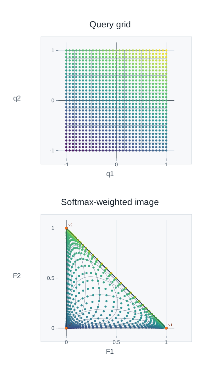
The output always lies in the triangle spanned by the three value vectors. The query vector does not choose fixed weights. It changes the scores, and the softmax rule changes all weights together.
A colored square grid of query vectors is shown next to its image under a softmax-weighted average map. The output points lie inside a triangle formed by three value vectors. The transformed grid bends and compresses toward different corners of the triangle.
Figure3.5.25.Square-grid visualization for an attention-style map \(\mathbf{q}\mapsto V^T\operatorname{softmax}(K\mathbf{q})\text{.}\) The output lies in the triangle spanned by the value vectors. The grid bends and compresses because the softmax weights depend nonlinearly on the query.
The entry \(S_{ij}\) compares the query for token \(i\) with the key for token \(j\text{.}\) A weighting rule, such as row-wise softmax, converts each row of \(S\) into weights. Write the resulting attention-weight matrix as \(A_{\mathrm{att}}\text{.}\) The attention output is
If \(A_{\mathrm{att}}\) were fixed, then \(V\mapsto A_{\mathrm{att}}V\) would be a linear map: each row of \(H\) would be a weighted average of rows of \(V\text{.}\) In attention, \(A_{\mathrm{att}}\) is not fixed. It is computed from \(X\) through \(Q\text{,}\)\(K\text{,}\) scores, and softmax. Thus the full rule \(X\mapsto H\) is generally nonlinear.
The Unit 3 question is local. Near one fixed input \(X_0\text{,}\) a nonlinear rule can be approximated by a linear map. After the entries of \(X\) and \(H\) are arranged as vectors, that local linear map is represented by a Jacobian matrix.
The matrices \(W_Q\text{,}\)\(W_K\text{,}\) and \(W_V\) are fixed. The matrices \(Q\text{,}\)\(K\text{,}\)\(V\text{,}\)\(S\text{,}\)\(A_{\mathrm{att}}\text{,}\) and \(H\) are computed from \(X\text{.}\)
The score matrix \(S=QK^T\) depends on \(X\) through \(Q\) and through \(K\text{.}\) The entries of \(S\) are dot products between query rows and key rows, and both sets of rows were computed from \(X\text{.}\)
If \(A_{\mathrm{att}}\) were fixed, then \(H=A_{\mathrm{att}}V\) would form weighted averages of the rows of \(V\text{.}\) This is linear in \(V\text{.}\)
In attention, \(A_{\mathrm{att}}\) is not fixed. The weights are computed from the input through scores and softmax. The values \(V\) also depend on \(X\text{.}\) Therefore the full rule \(X\mapsto H\) is generally nonlinear.
Near a fixed input \(X_0\text{,}\) the local linear approximation is represented by a Jacobian matrix after the entries of the input and output matrices are arranged as vectors.
Before asking whether a rule is linear, first say what is variable and what is fixed. The rule \(V\mapsto A_{\mathrm{att}}V\) is linear when \(A_{\mathrm{att}}\) is fixed. The attention rule \(X\mapsto A_{\mathrm{att}}(X)V(X)\) is generally nonlinear because the weights and values both depend on \(X\text{.}\)
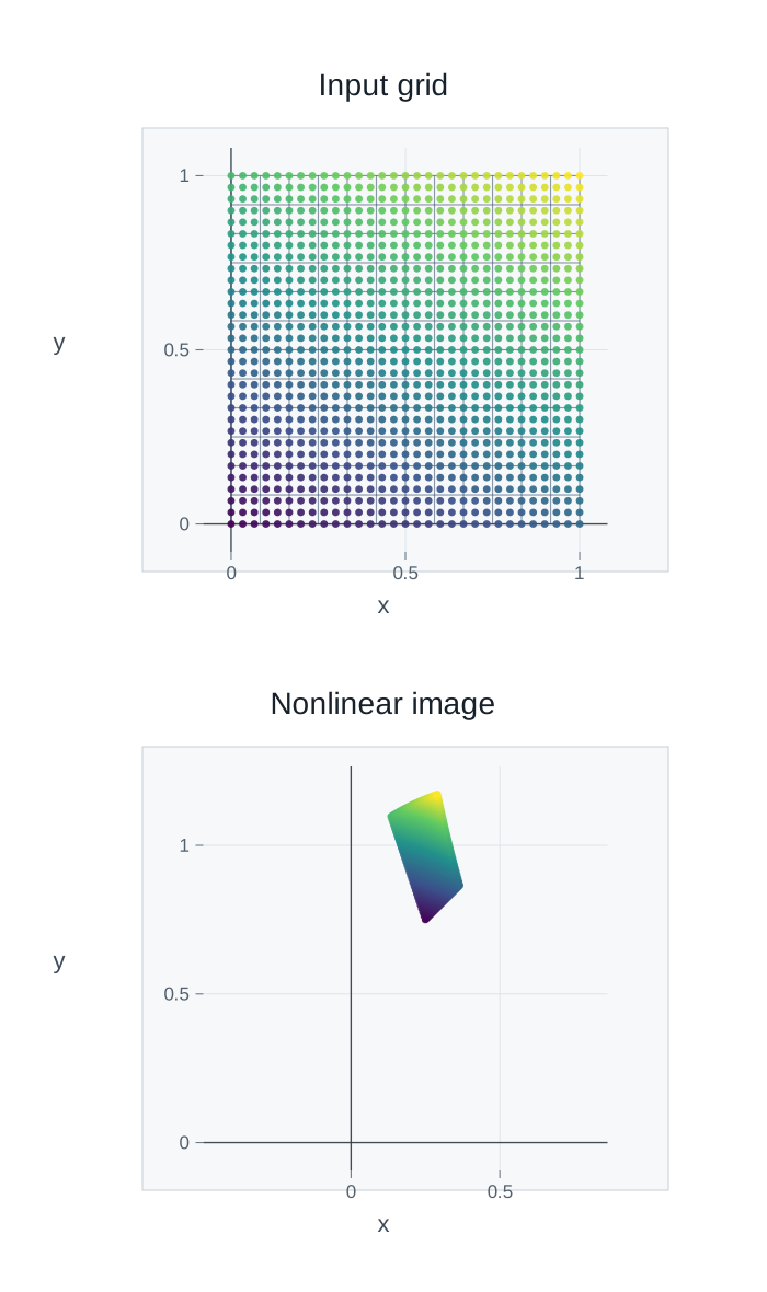
This unit used three square-grid visualizations: the nonlinear shear from Activity 3.1.4, the sigmoid block from Activity 3.5.20, and the attention-style softmax map from Activity 3.5.23.
Map B is the sigmoid block. Its Jacobian matrix near a base point has the form \(W_2D_{\mathbf{a}}W_1\text{,}\) where \(D_{\mathbf{a}}\) records the sigmoid derivatives at that base point. The local matrix can change from point to point because the sigmoid derivatives change.
Map C is the attention-style softmax map. Its outputs are weighted averages of the rows of \(V\text{,}\) so they stay inside the triangle spanned by the value vectors. The softmax weights depend on the input.