Lagrange multipliers and parallel gradients

Section 6.2 Lagrange multipliers and parallel gradients

Note 6.2.1. Lagrange multipliers as parallel gradients.

The Lagrange multiplier condition \(\nabla f(a)=\lambda\nabla g(a)\) means that, at a constrained optimum, the objective gradient is parallel to the constraint gradient. Equivalently, along the allowed tangent directions to the constraint, there is no first-order increase or decrease.

🔗

This uses four earlier ideas: dot products, orthogonality, level sets, and gradients.

🔗

We now discuss the method of Lagrange multipliers, which is a method of finding potential local minima and local maxima of a function on a hypersurface \(S\) in \(\R^n\) given as the level set of a function, i.e., when \(S = \{ \mathbf{x} \in \R^n: g(\mathbf{x}) = k \}\text{,}\) for some differentiable scalar-valued function \(g\) and some \(k \in \R\text{.}\)

🔗

Definition 6.2.2. Critical Points.

Consider a surface of the form \(S = \{ \mathbf{x} \in \R^n: g(\mathbf{x}) = k \}\text{,}\) where \(g\) is a differentiable scalar-valued function with \(\nabla g(\mathbf{x}) \neq 0\) for all \(\mathbf{x} \in S\text{.}\) If a point \(\mathbf{a} \in S\) is in the interior of the domain of a differentiable function \(f\text{,}\) then we say that \(\mathbf{a}\) is a constrained critical point of \(f\) on \(S\) if there exists \(\lambda \in \R\) such that

\begin{equation*} \nabla f(\mathbf{a}) = \lambda \nabla g(\mathbf{a})\text{.} \end{equation*}

Equivalently, define the Lagrangian function

\begin{equation*} \mathcal L(\mathbf{x},\lambda) = f(\mathbf{x})-\lambda(g(\mathbf{x})-k). \end{equation*}

Then \(\mathbf{a}\) is a constrained critical point exactly when there exists \(\lambda\in\mathbb R\) such that

\begin{equation*} \nabla_{\mathbf{x}}\mathcal L(\mathbf{a},\lambda)=\mathbf{0}, \qquad \frac{\partial \mathcal L}{\partial \lambda}(\mathbf{a},\lambda)=0. \end{equation*}

🔗

The method of Lagrange multipliers is a way of finding optima of a function \(f\) along a hypersurface \(S\) given as above. The method consists of finding all critical points of the function \(f\) on \(S\) (of which there are usually only finitely many). This consists of finding the solutions to the system of vector equations \(g(\mathbf{x}) = k\) and \(\nabla f(\mathbf{x}) = \lambda \nabla g(\mathbf{x})\text{.}\) The next theorem shows that any local extremum of \(f\) on \(S\) must occur at a critical point, so that the method of Lagrange multipliers will find these extrema.

🔗

Theorem 6.2.3.

Consider a surface

\begin{equation*} S=\{\mathbf{x}\in \mathbb R^n : g(\mathbf{x})=k\}, \end{equation*}

and assume \(\nabla g\) is nonzero on \(S\text{.}\) If a point \(\mathbf{a}\in S\) is a local extremum of a differentiable function \(f\) on \(S\text{,}\) and \(\mathbf{a}\) is an interior point of the domain of \(f\text{,}\) then \(\mathbf{a}\) is a constrained critical point of \(f\) on \(S\text{.}\)

🔗

In particular, if \(S\) is closed and bounded and \(f\) is continuous on \(S\text{,}\) then absolute extrema of \(f\) on \(S\) exist. Under the same differentiability and nonzero-gradient hypotheses, every absolute extremum of \(f\) on \(S\) is among the constrained critical points.

🔗

Why is this true?.

The idea is quite simple when sketched geometrically. In order for \(\mathbf{a}\) to be a local extremum for \(f\) on \(S\text{,}\) it must be true that for any unit vector \(\mathbf{v}\) in the tangent plane to \(S\) at a point \(\mathbf{a}\text{,}\) the directional derivative \(D_{\mathbf{v}} f(\mathbf{a})\) must be equal to \(0\) (or else travelling along \(S\) in the direction of \(\mathbf{v}\) or \(- \mathbf{v}\) will lead the function to increase or decrease, which contradicts the fact that \(\mathbf{a}\) is a local extrema). Recalling Definition 5.2.1, it follows that

\begin{equation*} \nabla f(\mathbf{a}) \cdot \mathbf{v} = 0 \end{equation*}

for any vector \(\mathbf{v}\) in the tangent plane to \(S\) at \(\mathbf{a}\text{,}\) which can only be true if \(\nabla f(\mathbf{a})\) is normal to the tangent plane to the surface \(S\) at \(\mathbf{a}\text{.}\) When \(S\) is equal to the level set of a function \(g\text{,}\) a normal vector to the tangent plane at \(\mathbf{a}\) is given by \(\nabla g(\mathbf{a})\text{.}\) So if \(\mathbf{a}\) is a local extremum of \(f\) on \(S\text{,}\) then \(\nabla f(\mathbf{a})\) and \(\nabla g(\mathbf{a})\) must be multiples of one another, i.e., it must be true that

\begin{equation*} \nabla f(\mathbf{a}) = \lambda \nabla g(\mathbf{a}) \end{equation*}

for some \(\lambda \in \R\text{,}\) i.e., so that \(\mathbf{a}\) is a constrained critical point of \(f\) on \(S\text{.}\)

🔗

The final statement follows from the extreme value theorem: if \(S\) is closed and bounded and \(f\) is continuous on \(S\text{,}\) then absolute extrema exist, and any absolute extremum is also a local extremum on \(S\text{.}\) The first part of the theorem then shows that such a point must be a constrained critical point.

🔗

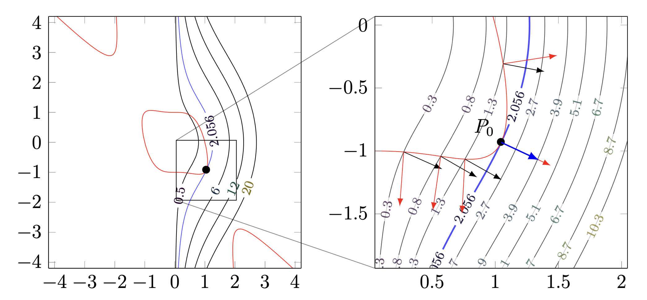
Contour and constraint diagram showing normal vectors at a constrained critical point. — Figure 6.2.4. Suppose we are optimizing a function, whose contours are the red curves in this diagram, subject to a given constraint which restricts our values to lie on the blue curve in the diagram. Then the critical points along this curve occur when the normal vectors to the red curve and the blue curve agree. From: Stanford’s MATH 51 textbook
🔗

Activity 6.2.1.

Find the absolute extrema of \(f(x,y) = 3x + y\) subject to the constraint \(x^2 + y^2 = 10\text{.}\)

🔗

Solution.

Write \(g(x,y) = x^2 + y^2\text{.}\) Then we are finding extrema of \(f\) on the surface

\begin{equation*} S = \{ (x,y): g(x,y) = 10 \}\text{.} \end{equation*}

We calculate that

\begin{equation*} \nabla f(x,y) = (3,1) \quad\text{and}\quad \nabla g(x,y) = (2x,2y)\text{.} \end{equation*}

So the constrained critical points of \(f\) on \(S\) are the points \((x,y) \in S\) for which there exists \(\lambda\) such that

\begin{equation*} (3,1) = \lambda (2x,2y)\text{,} \end{equation*}

i.e., the points that satisfy the three equations

\begin{align*} x^2 + y^2 \amp = 10\\ 2 \lambda x = 3\\ 2 \lambda y = 1\text{.} \end{align*}

If the second and third equation holds, then \(\lambda\) cannot be zero, and we can divide both sides of the equation by \(\lambda\) to obtain that \(x = 3/2\lambda\) and \(y = 1/2\lambda\text{.}\) Substituting this into the first equation, we find that

\begin{equation*} (3/2\lambda)^2 + (1/2\lambda)^2 = 10\text{,} \end{equation*}

which simplifies to \(1/4 = \lambda^2\text{,}\) so either \(\lambda = 1/2\) or \(\lambda = -1/2\text{.}\) If \(\lambda = 1/2\text{,}\) then \(x = 3\) and \(y = 1\text{,}\) and if \(\lambda = -1/2\text{,}\) then \(x = -3\) and \(y = -1\text{.}\) So the two points \((3,1)\) and \((-3,-1)\) are the two constrained critical points of \(f\) on \(S\text{.}\) Since \(S\) is a circle, and is closed and bounded, the absolute maximum and minimum occur among these two points. We have

\begin{equation*} f(3,1) = 10 \quad\text{and}\quad f(-3,-1) = -10\text{,} \end{equation*}

so \((3,1)\) is the absolute maximum of \(f\) on \(S\text{,}\) and \((-3,-1)\) is the absolute minimum of \(f\) on \(S\text{.}\)

🔗

Activity 6.2.2.

Find the absolute extrema of the function \(f(x,y,z) = x^2 + 2y^2 + 3z^2\text{,}\) subject to the constraint \(x^2 + y^2 + z^2 = 1\text{.}\)

🔗

Solution.

Let \(g(x,y,z) = x^2 + y^2 + z^2\text{.}\) Then \(\nabla f(x,y,z) = (2x,4y,6z)\) and \(\nabla g(x,y,z) = (2x,2y,2z)\text{.}\) A point \((x,y,z)\) is a constrained critical point of \(f\) on the sphere \(S = \{ (x,y,z): x^2 + y^2 + z^2 = 1 \}\) only when there exists \(\lambda \in \R\) so that the two equations

\begin{equation*} \nabla f(x,y,z) = \lambda \nabla g(x,y,z) \quad\text{and}\quad x^2 + y^2 + z^2 = 1 \end{equation*}

both hold, which expands to the four equations

\begin{gather*} 2x = \lambda 2x\\ 4y = \lambda 2y\\ 6z = \lambda 2z\\ x^2 + y^2 + z^2 = 1\text{.} \end{gather*}

Since \(x^2 + y^2 + z^2 = 1\text{,}\) either \(x \neq 0\) (and dividing the first equation by \(x\) we obtain \(\lambda = 1\)), \(y \neq 0\) (and dividing the second equation we obtain \(\lambda = 2\)), or \(z \neq 0\) (and dividing the third equation by \(z\) gives \(\lambda = 3\)). When \(\lambda = 1\text{,}\) the first equation automatically holds, and the second and third equation can only hold when \(y = z = 0\text{.}\) Thus the fourth equation becomes \(x^2 = 1\text{,}\) so \(x = \pm 1\text{.}\) Similarly, when \(\lambda = 2\) we have \(x = z = 0\) and \(y = \pm 1\text{,}\) and when \(\lambda = 3\) we have \(x = y = 0 \) and \(z = \pm 1\text{.}\) So the function \(f\) has six constrained critical points on \(S\text{,}\) at the points \((\pm 1,0 ,0)\text{,}\) \((0,\pm 1, 0)\text{,}\) and \((0,0,\pm 1)\text{.}\) We have

\begin{equation*} f(\pm 1,0,0) = 1 \quad f(0,\pm 1, 0) = 2 \quad\text{and}\quad f(0,0,\pm 1) = 3\text{.} \end{equation*}

So the absolute minima of \(f\) occur at \((\pm 1, 0, 0)\text{,}\) and the absolute maxima of \(f\) occur at \((0,0,\pm 1)\text{.}\)

🔗

Prev Top Next