Unit 1 and Unit 2 studied maps of the form \(\mathbf{x}\mapsto A\mathbf{x}\text{.}\) We now allow more general rules. The output may be a scalar or a vector.
A vector-valued map is usually written \(F:\R^n\to\R^m\text{.}\) A scalar-valued function is usually written \(f:\R^n\to\R\text{.}\) Any vector-valued map \(F:\R^n\to\R^m\) has \(m\) component functions, or coordinate functions, the scalar-valued functions \(F_1,\dots,F_m:\R^n\to\R\) such that
More generally, vector-valued and scalar-valued functions may only be defined on a subset of vectors in \(\R^n\text{,}\) rather than defined everywhere, so their domain may be a proper subset of \(\R^n\text{.}\)
In other words, a scalar-valued function takes in an input and outputs scalars, and a vector-valued function takes in an input and outputs vectors (recall Definition 1.1.1).
Activity3.1.2.Vector length as a scalar-valued function (U3-LO1).
If \(\mathbf{x}\) is a point in \(\R^n\text{,}\) recall the length of \(\mathbf{x}\text{,}\) denoted \(\| \mathbf{x} \|\text{,}\) from Definition 1.1.4. The length of a vector defines a scalar-valued function from \(\R^n\) to \(\R\text{.}\) Find two different vectors with the same length. What does this say about whether the output determines the input?
There are many different choices one could make here. For instance, the vector \((3,4)\) and the vector \((5,0)\) both have the same length. Other examples are the vectors \((1,2)\) and \((-1,2)\text{.}\)
Activity3.1.3.Component functions of a matrix map (U3-LO1).
Let \(A\) be an \(m \times n\) matrix. The linear map (recall Definition 1.3.27) \(T: \R^n \to \R^m\) defined by \(T(\mathbf{x}) = T_A(\mathbf{x}) = A\mathbf{x}\) is a vector-valued map. Each component function is a row dot product.
If \(\mathbf{a}_1, \dots, \mathbf{a}_m\) are the rows of \(A\text{,}\) viewed as vectors in \(\R^n\text{,}\) and \(T_1, \dots, T_m\) are the component functions of \(T\text{,}\) then for each \(j\text{,}\) express the function \(T_j\) in terms of the row \(\mathbf{a}_j\text{.}\)
which defines a linear map \(T_A: \R^3 \to \R^2\text{.}\) Compute its component functions for a general input \(\mathbf{x}\text{,}\) and its output for the specific input \(\mathbf{x} = (3, -1, 2)\text{.}\)
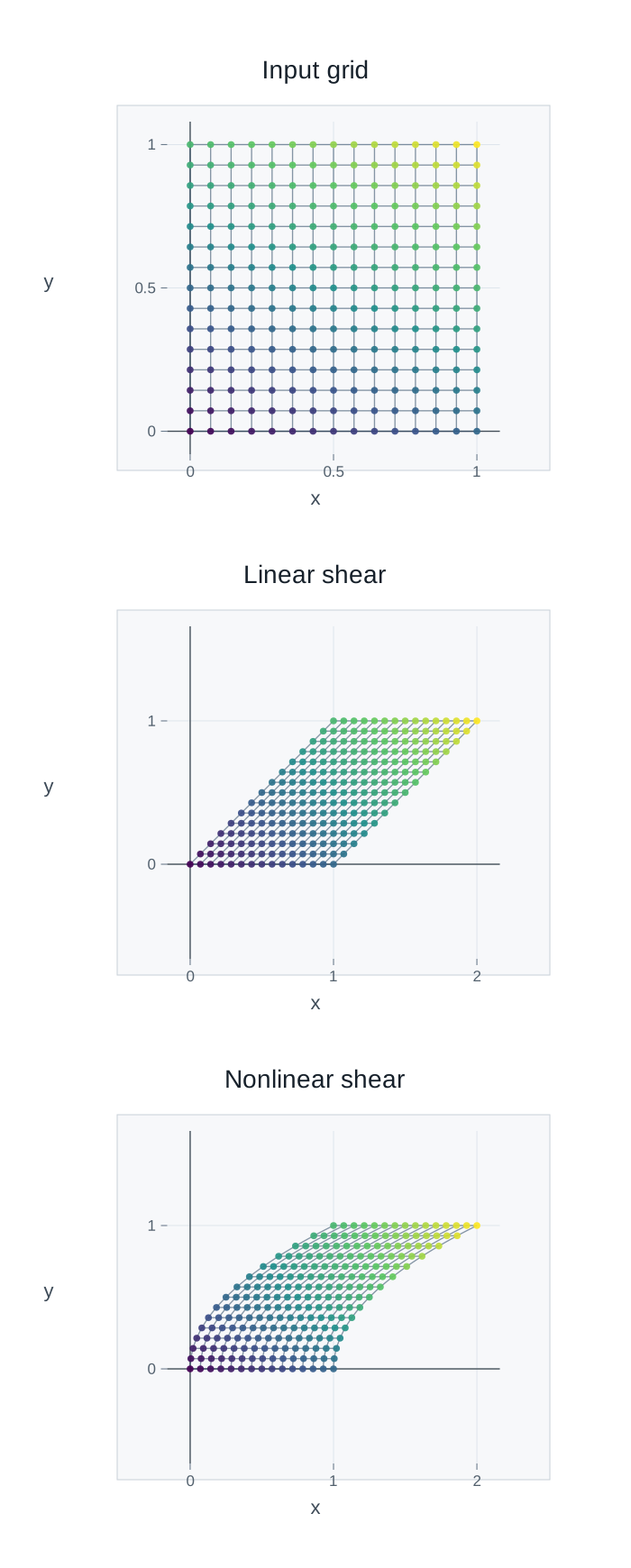
A matrix sends grid lines to grid lines. A nonlinear map can bend grid lines. The square-grid visualization samples points and grid lines, not only the corners.
The four corners have the same images under \(F\) and under \(T(x,y)=(x+y,y)\text{.}\) The midpoint does not. A grid includes edge and interior points, so it can show bending that the four corners miss.
A square-grid diagram keeps track of input points and output points at the same time. The color identifies the original input point. The grid lines show how nearby input points move.
A colored grid in the unit square is shown next to its images under a linear shear and a nonlinear shear. The linear shear sends the grid to straight slanted grid lines. The nonlinear shear bends some grid lines even though the four corners match the linear shear.
Figure3.1.8.Square-grid visualization for \(T(x,y)=(x+y,y)\) and \(F(x,y)=(x+y^2,y)\text{.}\) The color identifies the original input point. The two maps agree on the four corners, but the nonlinear map bends grid lines.
The domain of a function is the set of all inputs for that function, and the range is the set of all possible outputs. More formally, if a function \(f\) takes inputs from a set \(X\) and outputs elements in a set \(Y\text{,}\) then the domain of \(f\) is the set \(X\text{,}\) and the range is the set of all \(y \in Y\) for which \(y = f(x)\) for some \(x \in X\text{,}\) which we might write in set notation as \(\{ y \in Y: y = f(x)\ \text{for some}\ x \in X \}\text{.}\)
In calculus, we often define the domain of a function \(f\)implicitly, by defining \(f\) in terms of an expression, and then letting the domain of \(f\) be the set of all values which, when substituted into that expression, lead to a well-defined quantity. For instance, we might discuss ‘the function’ \(f(x,y) = x/y\text{,}\) by which we mean the function with domain \(\{ (x,y) \in \R^2 : y \neq 0 \}\) and range \(\R\text{.}\)
The range contains only outputs actually attained by the function, while the co-domain, defined in Linear and affine maps, is the specified output set and may be larger than the range.
For scalar-valued functions of two variables, domains and level curves are subsets of the plane. These pictures help us see where a function is defined and how its outputs change.
The expression that defines the function \(f\) consists of the sum of two terms, and so to find the domain of \(f\text{,}\) we must identify where both terms are well defined.
The term \(\ln(y - x^2)\) is well defined when the input to \(\ln\) is positive, i.e., when \(y - x^2 > 0\text{.}\) We may rearrange this inequality to read \(y > x^2\)
So \(f\) is well-defined when both \(y > x^2\) and when \(x \geq 0\text{,}\) and so the domain of \(f\) is the set of all points \((x,y)\) such that \(x \geq 0\) and \(y > x^2\text{.}\) Using set notation, we can also write the domain as the set
\begin{equation*}
\{ (x,y) \in \R^2: x \geq 0\ \text{and}\ y > x^2 \}\text{.}
\end{equation*}
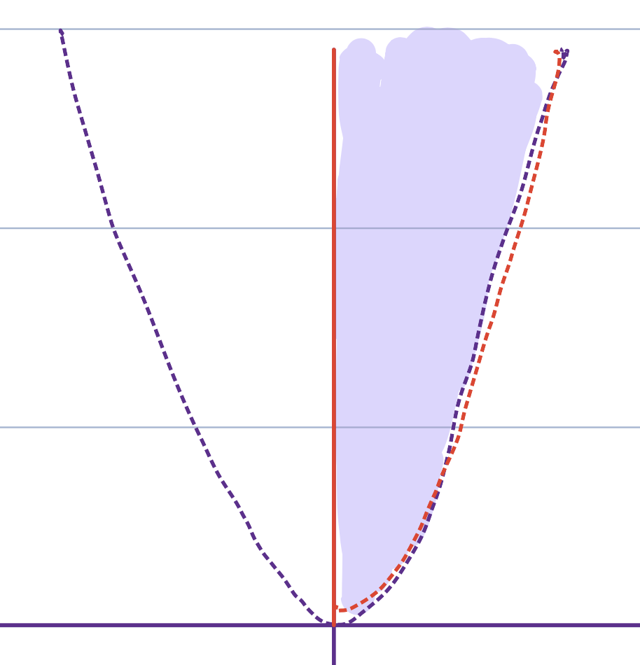
The set is the region in the plane bounded from below by the parabola \(y = x^2\text{,}\) and on the left by the \(y\)-axis, as depicted in Figure 3.1.11.
The figure shows coordinate axes with a vertical boundary at \(x=0\) and an upward-opening parabola \(y=x^2\text{.}\) The shaded purple region lies to the right of the \(y\)-axis and above the parabola. The drawing emphasizes that the domain requires both \(x\geq 0\) and \(y>x^2\text{.}\)
The expression defining the function \(f\) consists of the product of \(e^x\) and \(\sin y\text{,}\) and so \(f\) is well-defined precisely when \(e^x\) and \(\sin y\) are both well-defined. Both expressions are well-defined for all inputs. And so the domain of \(f\) is the set \(\R^2\text{.}\)
The expression defining \(f\) is a fraction with numerator \(\sqrt{x}\) and denominator \(\sqrt{y}\text{.}\) The expression is therefore well-defined when both the numerator and denominator are well defined, and when the denominator is non-zero.
The numerator \(\sqrt{x}\) is well-defined when \(x \geq 0\text{.}\) The denominator \(\sqrt{y}\) is well-defined when \(y \geq 0\text{,}\) and is non-zero when \(y > 0\text{.}\)
So the domain of \(f\) is the set of all \((x,y) \in \R^2\) with \(x \geq 0\) and \(y > 0\text{,}\) or in set notation, the set
\begin{equation*}
\{(x,y) \in \mathbb{R}^2 : x \geq 0\ \text{ and }\ y > 0\}\text{.}
\end{equation*}
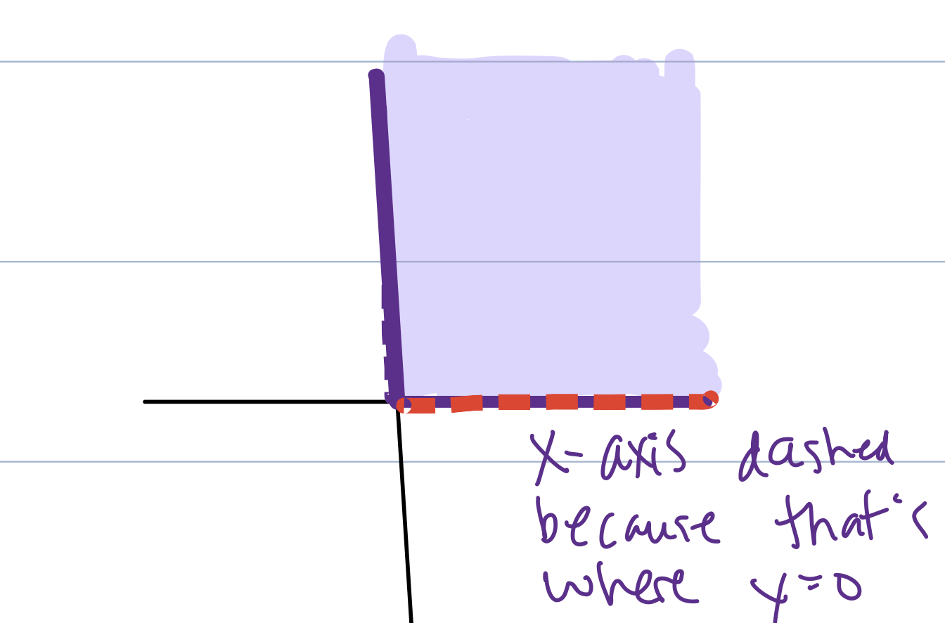
This set is the first quadrant in the \(xy\)-plane, including the positive \(y\)-axis, but excluding the origin and the positive \(x\)-axis. See Figure 3.1.12.
The coordinate plane is shaded purple in the region with \(x\geq 0\) and \(y>0\text{.}\) The \(y\)-axis is included as part of the boundary, while the \(x\)-axis is drawn as a dashed red boundary to show it is excluded. A handwritten note points out that the dashed boundary is where \(y=0\text{.}\)
When \(f\) is a scalar-function of two variables, the graph of \(f\) is a set of triples \((x,y,f(x,y))\text{,}\) and thus a subset of \(\R^3\text{,}\) and can therefore be visualized as a surface. See Figure 3.1.14 for a picture of the graph of the function \(f(x,y) = x e^{-x^2-y^2}\text{.}\)
The figure shows a 3D coordinate system with a red mesh surface for \(z=x e^{-x^2-y^2}\text{.}\) The surface rises to a rounded ridge on the positive \(x\) side and falls to a matching trough on the negative \(x\) side. Away from the origin, the surface flattens toward the \(xy\)-plane.
A level curve of a scalar function \(f\) of two variables is the curve consisting of pairs \((x,y)\) satisfying the equation \(f(x,y) = c\text{,}\) for some \(c \in \R\text{.}\) A contour plot is a sketch in \(\R^2\) depicting level curves of a function \(f\) for many different values of \(c\text{.}\)
The different values of \(c\) which are chosen to be depicted in a contour plot are often (but not always) obtained by varying \(c\) by a common difference, obtaining ‘consecutive’ level sets.
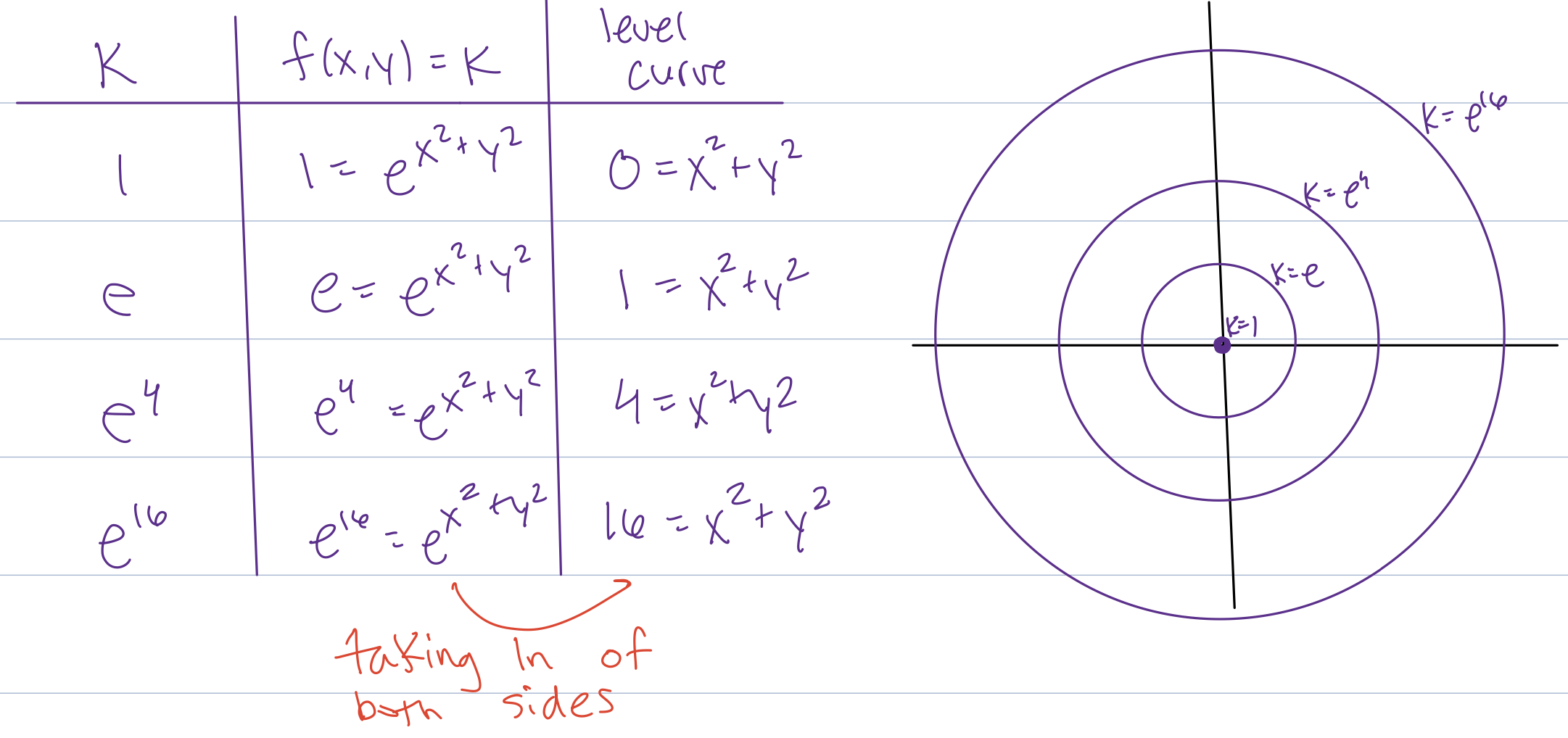
The left side lists level values such as \(1\text{,}\)\(e\text{,}\)\(e^4\text{,}\) and \(e^9\) with the corresponding equations for \(x^2+y^2\text{.}\) The right side shows concentric circles centered at the origin in the \(xy\)-plane. Larger level values correspond to circles farther from the origin.
This short section supplies local language used in derivative and optimization statements: balls, limits, continuity, interior points, boundary points, closed sets, and bounded sets.
Recall the definition of a limit from single-variable calculus. For a function \(f: \R \to \R\) and \(a,b \in \R\text{,}\) the equation
\begin{equation*}
\lim_{x \to a} f(x) = b
\end{equation*}
holds if for each \(\varepsilon > 0\text{,}\) there is \(\delta > 0\) so that if \(0 \lt |x - a| \lt \delta\text{,}\) then \(|f(x) - b| \lt \varepsilon\text{.}\) We can interpret this statement geometrically as follows: for any open interval \(J\) centered at \(b\text{,}\) there is an open interval \(I\) centered at \(a\) so that \(f\) maps points in \(I\text{,}\) excluding \(a\) itself, into \(J\text{.}\)
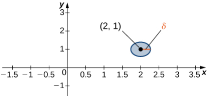
Consider a point \((a,b) \in \mathbb{R}^2\text{.}\) The \(\delta\)-disk centered at point \((a,b)\) is the region of \(\R^2\) bounded by the circle of radius \(\delta\) centered at \((a,b)\text{,}\) i.e., the set
The \(xy\)-plane is shown with a small blue disk centered at the black point \((2,1)\text{.}\) An arrow labeled \(\delta\) points from the center to the edge of the disk, indicating the disk’s radius. The disk lies near the positive \(x\)-axis and above the positive \(y\)-axis tick mark \(1\text{.}\)
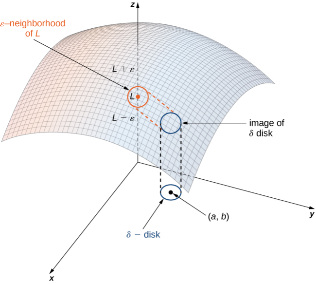
will then hold precisely when, for each open interval \(I\) centered at \(L\text{,}\) there is a \(\delta\) disk centered at \((a,b)\) so that all points in this disk which are also contained in the domain of \(f\text{,}\) excluding the point \((a,b)\) itself, are mapped by \(f\) into \(I\text{.}\)
A 3D surface is drawn above the \(xy\)-plane, with a disk of radius \(\delta\) centered at \((a,b)\) in the domain. A vertical guide from the disk reaches the surface near the height \(L\text{.}\) A shaded band labeled as an \(\varepsilon\)-neighborhood of \(L\) indicates that the image of the disk stays between \(L-\varepsilon\) and \(L+\varepsilon\text{.}\)
Using vector-notation (recalling Definition 1.1.4), we can write a \(\delta\)-disk centered at a point \(\mathbf{x}_0 \in \R^2\) as the set of points \(\mathbf{x} \in \R^2\) so that
if for each \(\varepsilon > 0\text{,}\) there is \(\delta > 0\) so that for any points in the domain of \(f\) with \(0 \lt \| \mathbf{x} - \mathbf{x}_0 \| \lt \delta\text{,}\) the inequality \(|f(\mathbf{x}) - L| \lt \varepsilon\) holds.
In order for the limit of \(f\text{,}\) when it exists, to be unique, the point \(\mathbf{x}_0\) must have the property that the domain of \(f\) contains a point other than \(\mathbf{x}_0\) in any \(\delta\)-ball centered at \(\mathbf{x}_0\text{.}\) This is only a small issue, since every point in the domain of any of the functions that naturally occur in calculus have this property.
Recall from the calculus of a single variable that a function \(f: \R \to \R\) is continuous at a point \(a\) when \(\lim_{x \to a} f(x) = f(a)\text{,}\) i.e., when the limit on the left hand side exists and is equal to the right hand side. The continuity of functions of several variables is defined in exactly the same way.
A scalar-valued function \(f\) is continuous at a point \(\mathbf{x}_0\) in its domain if the limit of \(f\) as \(\mathbf{x} \to \mathbf{x}_0\) exists, and
Definition3.1.26.Interior, boundary, and closed sets.
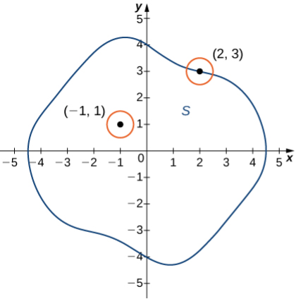
Let \(S\) be a subset of \(\R^n\text{.}\) Then a point \(\mathbf{x}_0 \in S\) is an interior point if there is a \(\delta\)-ball centered at \(\mathbf{x}_0\) completely contained in \(S\text{.}\) A point \(\mathbf{x}_0 \in \R^n\) is a boundary point if every ball centered at \(\mathbf{x}_0\) contains at least one point of \(S\) and at least one point outside \(S\text{.}\) The set of all boundary points of a set \(S\) is called the boundary of the set \(S\text{.}\)
The set \(S\) is drawn as an irregular closed blue curve in the coordinate plane. The point \((-1,1)\) appears inside the curve with a small orange neighborhood around it. The point \((2,3)\) lies on the boundary, and its small orange neighborhood crosses both inside and outside the set.
Note that a boundary point of a set \(S\)need not be contained in the set \(S\). For example, the \(\delta\)-disk defined in this section does not contain its circular boundary. A set that contains its boundary is called closed.
A set \(S \subset \R^n\) is called closed if it contains its boundary. A set \(S \subset \R^n\) is bounded if it is contained in some ball centered at the origin, or equivalently if all points of \(S\) lie within some fixed distance of the origin.