An \(n\)-vector is an ordered list of \(n\) scalars, often written in the form \(\mathbf{v} = (v_1,v_2,\ldots,v_n)\text{.}\) The collection of all \(n\)-vectors is denoted \(\R^n\text{.}\)
It is customary to use bold letters for variables, such as \(\mathbf{v}\) or \(\mathbf{w}\text{,}\) to represent vectors. We let \(\mathbf{0}\) denote the vector \((0,\dots,0)\) consisting only of zeros. Two vectors \(\mathbf{v}\) and \(\mathbf{w}\) are equal if they have the same number of entries and all the corresponding entries are equal. A point in \(n\)-dimensional space can also be identified with an ordered list of \(n\) numbers using Cartesian coordinates. When referring specifically to a point \(P\text{,}\) we write \(P(x_1,x_2,\ldots,x_n)\) to indicate its coordinates.
SubsectionVectors as displacements in space: building intuition
Vectors can be used to represent displacements between points in space. The vector \(\mathbf{v}=(v_1,v_2,v_3)\) represents the displacement from \(P(x_1,y_1,z_1)\) to \(Q(x_2,y_2,z_2)\text{,}\) where \(x_2 = x_1 + v_1\text{,}\)\(y_2 = y_1 + v_2\text{,}\) and \(z_2 = z_1 + v_3\text{.}\) This vector is also written as \(\overrightarrow{PQ}\text{.}\) Because vectors often indicate displacements, they are drawn pictorially as arrows starting at a point, and ending where that point is displaced by the vector.
Three coordinate axes labeled \(x\text{,}\)\(y\text{,}\) and \(z\) meet at an origin. A thick arrow labeled \(\mathbf{v}\) starts at the red point \(P\) and ends at the red point \(Q\text{,}\) showing the displacement from \(P\) to \(Q\text{.}\)
If \(\mathbf{v} = (v_1,v_2)\) was the displacement, then we would have \((1 + v_1, 2 + v_2) = (5,7)\text{,}\) i.e., so that \(1 + v_1 = 5\) and \(2 + v_2 = 7\text{.}\) Solving these equations gives \(v_1 = 4\) and \(v_2 = 5\text{,}\) so that the displacement vector is \(\mathbf{v} = (4,5)\text{.}\)
Let \(\mathbf{v} = (x,y)\) be an arbitrary \(2\)-vector. Consider a triangle with vertices \(P(0,0)\text{,}\)\(Q(x,0)\text{,}\) and \(R(x,y)\) (see Figure 1.1.6).
The figure shows \(x\)- and \(y\)-axes with a vector \(\mathbf{v}\) drawn from \(P(0,0)\) to \(R(x,y)\text{.}\) A horizontal segment from \(P\) to \(Q(x,0)\) and a vertical segment from \(Q\) to \(R\) form a right triangle whose hypotenuse is the vector.
Figure1.1.6.A triangle with vertices \(P(0,0)\text{,}\)\(Q(x,0)\text{,}\) and \(R(x,y)\text{,}\) drawn to determine the length of the line-segment upon which a \(2\)-vector is based.
This triangle is right-angled (the two legs are horizontal and vertical), and the hypotenuse is the line-segment upon which the vector \(\mathbf{v}\) is built. The length of the leg from \(P(0,0)\) to \(Q(x,0)\) is \(|x|\text{,}\) and the length of the leg from \(Q(x,0)\) to \(R(x,y)\) is \(|y|\text{.}\) By Pythagoras’ theorem, we conclude that the length of the hypotenuse is
In a calculus course, you may have mostly seen a vector as a displacement, but in this course it can also be a row of data or a list of model parameters, among other important applications. The same operations below will later compare documents, tokens, and feature vectors.
The sum of two \(n\)-vectors \(\mathbf{v} = (v_1,\dots,v_n)\) and \(\mathbf{w} = (w_1,\dots,w_n)\text{,}\) denoted \(\mathbf{v} + \mathbf{w}\text{,}\) is the vector given by the tuple \((v_1 + w_1, \dots, v_n + w_n)\text{.}\)
The sum of two vectors can be illustrated pictorially as in Figure 1.1.9 by drawing the parallelogram with the vectors placed along two sides of the parallelogram.
A blue vector \(\mathbf{v}\) and a red vector \(\mathbf{w}\) start at the origin. Dashed copies of each vector are translated to the tip of the other vector, and both translated arrows meet at a shared endpoint. A green arrow from the origin to that endpoint is labeled \(\mathbf{v}+\mathbf{w}\text{.}\)
If \(\mathbf{v} = (v_1,\cdots,v_n)\) is an \(n\)-vector and \(t \in \R\) is a scalar, we let \(t \mathbf{v}\) denote the vector \((tv_1, \cdots, tv_n)\text{,}\) i.e., multiplying each entry of the vector \(\mathbf{v}\) by \(t\text{.}\)
is a linear combination of \(\mathbf{v}_1,\ldots,\mathbf{v}_k\text{.}\) The scalars \(c_1,\ldots,c_k\) are the coefficients of the linear combination. If \(c_i\ge 0\) for all \(i\) and \(c_1+\cdots+c_k=1\text{,}\) then the linear combination is a convex combination.
Let \(\mathbf{v}_1=(10,0)\text{,}\)\(\mathbf{v}_2=(0,10)\text{,}\) and \(\mathbf{v}_3=(10,10)\text{.}\) Let \(\alpha_1=1/4\text{,}\)\(\alpha_2=1/4\text{,}\) and \(\alpha_3=1/2\text{.}\) Compute \(\alpha_1\mathbf{v}_1+\alpha_2\mathbf{v}_2+\alpha_3\mathbf{v}_3\text{.}\)
Thus, \(\mathbf{u}-\mathbf{v}\) is a linear combination of \(\mathbf{u}\) and \(\mathbf{v}\) with coefficients \(1\) and \(-1\text{.}\) For example, if \(\mathbf{u}=(4,1)\) and \(\mathbf{v}=(1,3)\text{,}\) then
Geometrically, \(-\mathbf{v}\) has the same length as \(\mathbf{v}\) but points in the opposite direction. We can therefore use the parallelogram construction from Figure 1.1.9 with \(\mathbf{u}\) and \(-\mathbf{v}\text{,}\) as shown on the left in Figure 1.1.14. Equivalently, when \(\mathbf{u}\) and \(\mathbf{v}\) start at the same point, the arrow from the tip of \(\mathbf{v}\) to the tip of \(\mathbf{u}\) represents \(\mathbf{u}-\mathbf{v}\text{.}\) Here, it is the displacement from \(P(1,3)\) to \(Q(4,1)\text{,}\) shown on the right.
On the left, a blue arrow \(\mathbf{u}=(4,1)\) and a red arrow \(-\mathbf{v}=(-1,-3)\) start at the same point. Dashed translated copies complete a parallelogram, whose green diagonal is \(\mathbf{u}-\mathbf{v}=(3,-2)\text{.}\) On the right, blue \(\mathbf{u}\) and red \(\mathbf{v}\) start at the origin and end at \(Q(4,1)\) and \(P(1,3)\text{,}\) respectively. A green arrow from \(P\) to \(Q\) represents the same difference \(\mathbf{u}-\mathbf{v}\text{.}\)
Figure1.1.14.The difference \(\mathbf{u}-\mathbf{v}\) as the sum \(\mathbf{u}+(-\mathbf{v})\) (left) and as the displacement from the tip of \(\mathbf{v}\) to the tip of \(\mathbf{u}\) (right).
Geometrically, the dot product of two vectors is a quantity which is related to the angle between the two vectors \(\mathbf{v}\) and \(\mathbf{w}\text{.}\) If we draw the two vectors as arrows with the same starting point, then they form an angle on the plane containing both vectors, and the angle \(\theta\) is given below.
The dot product can be thought of as a measure of the similarity between two vectors. Suppose \(\theta\) is the angle between two vectors \(\mathbf{v}\) and \(\mathbf{w}\text{:}\)
If \(\theta\) is close to zero, then the two vectors are close to pointing in the same direction. Since \(\cos(0^\circ) = 1\text{,}\) this occurs precisely when
If \(\theta\) is close to \(180^\circ\text{,}\) then the two vectors are close to pointing in opposite directions. Since \(\cos(180^\circ) = -1\text{,}\) this occurs precisely when
If \(\theta\) is close to \(90^\circ\text{,}\) the two vectors are close to pointing at right angles. Since \(\cos(90^\circ) = 0\text{,}\) this occurs precisely when
It ranges between \(-1\) and \(1\text{,}\) and measures the degree to which the two vectors point in the same, or opposite, directions. This terminology is especially common in certain areas of data science.
A dashed coordinate grid is shown with \(x\)- and \(y\)-axes. A blue arrow from the origin ends at \((1,2)\text{,}\) while a longer red arrow from the origin ends at \((\sqrt{3}+2, 2\sqrt{3}-1)\text{.}\) The two arrows represent the vectors used in the cosine-similarity activity.
As illustrated in Figure 1.1.14, \(\mathbf{u}-\mathbf{v}\) points from the tip of \(\mathbf{v}\) to the tip of \(\mathbf{u}\) when the two vectors start at the same point. Its Euclidean norm therefore measures how far apart those endpoints are. For the vectors in Example 1.1.13,
Vectors can represent quantities other than displacements. The entries of a vector can record measurements, counts, samples, or features. The meaning of a vector depends on what its coordinates represent.
measured attributes such as size, price, weight, or rating
The same vector operations can have different interpretations. A sum can add purchases, add word counts, or add two time series. A scalar multiple can rescale an image, double a portfolio, or change units. A dot product can produce a score. A distance can compare two feature vectors. Cosine similarity compares direction after normalization.
Compute the cosine similarities and Euclidean distances between \(\mathbf{q}\) and each \(\mathbf{D}_i\text{.}\) Rank the documents from most to least similar by cosine similarity and from closest to farthest by Euclidean distance.
The vector \(\mathbf{D}_1\) points in exactly the same direction as \(\mathbf{q}\) because \(\mathbf{D}_1=3\mathbf{q}\text{.}\) The vector \(\mathbf{D}_2\) shares the word “linear” with the query but also contains “matrix”. The vector \(\mathbf{D}_3\) contains only “matrix”, so it is orthogonal to the query.
In the previous activity, \(\mathbf{D}_1\) is most similar to the query by cosine similarity but farthest from it by Euclidean distance; \(\mathbf{D}_2\) is closest by Euclidean distance. The two measures select different documents because cosine similarity compares direction after normalization, while Euclidean distance also depends on vector length.
Activity1.1.25.The same rankings in code (U1-LO2, U1-LO8).
The following code repeats the cosine-similarity and Euclidean-distance rankings from Activity 1.1.24. We compute the cosine similarities between the query and each document, then the Euclidean distances by taking the norm of each difference.
The first tuple gives the cosine similarities and the second gives the Euclidean distances, each in the order \(\mathbf{D}_1\text{,}\)\(\mathbf{D}_2\text{,}\)\(\mathbf{D}_3\) relative to \(\mathbf{q}\text{.}\) Smaller distances mean closer documents.
The score for \(\mathbf{D}_2\) is score2. The expression D1 @ q computes \(\mathbf{D}_1\cdot\mathbf{q}\text{.}\) Since score1 is largest, \(\mathbf{D}_1\) is most similar to the query.
The line distance2 = np.linalg.norm(D2 - q) computes \(\|\mathbf{D}_2-\mathbf{q}\|\text{.}\) The distances are \(2\sqrt{2}\text{,}\)\(\sqrt{2}\text{,}\) and \(\sqrt{6}\text{,}\) respectively, so the ranking from closest to farthest is \(\mathbf{D}_2\text{,}\) then \(\mathbf{D}_3\text{,}\) then \(\mathbf{D}_1\text{.}\) By cosine similarity, the ranking is \(\mathbf{D}_1\text{,}\) then \(\mathbf{D}_2\text{,}\) then \(\mathbf{D}_3\text{.}\) Thus, \(\mathbf{D}_1\) is first by cosine similarity, while \(\mathbf{D}_2\) is first by Euclidean distance.
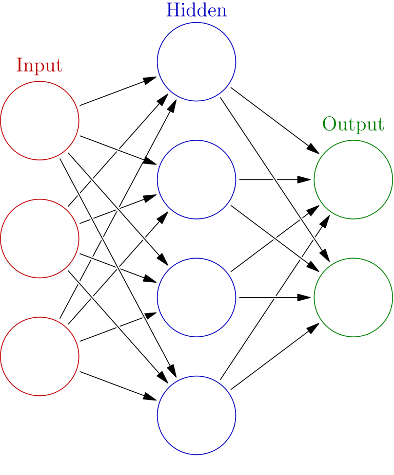
A neural network is a function built from layers. A layer takes numbers as input, combines them using weights, applies a rule, and sends output numbers to the next layer. In many neural networks, the input and output of a layer are vectors. The weights are adjusted from data during training.
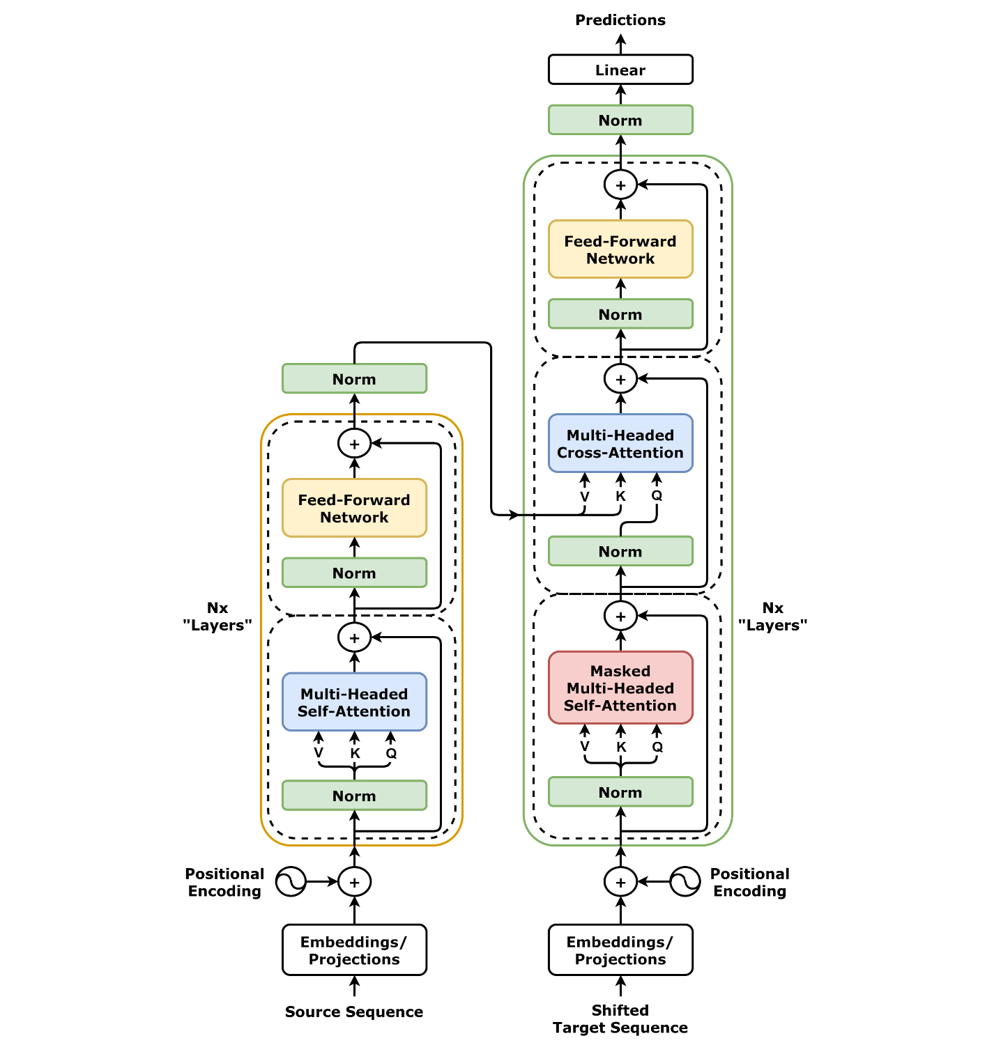
A transformer is a neural-network architecture for sequences. In a language model, text is first broken into tokens. A token can be a word, part of a word, punctuation mark, or other text fragment. Each token position carries a vector.
A transformer layer produces a new vector at each token position. The token itself does not change; its vector becomes context-dependent. In the phrase “small red bird”, the new vector at the bird position can gather information from “small” and “red”. In a next-token model, the vector at this final position can then help predict what comes next.
For one output position, its query is used to decide which positions are relevant. Each token has a key used in that comparison and a value containing the information it can contribute. Queries and keys determine the weights; values are what get averaged. Every position has all three roles, but the next activity computes only the attention output at the bird position.
Three red input nodes are arranged vertically on the left, four blue hidden-layer nodes appear in the center, and two green output nodes appear on the right. Black arrows connect each input node to the hidden layer, and gray arrows connect the hidden layer to the outputs, showing information moving left to right through the network.
The diagram has two vertical stacks: an encoder stack for a source sequence on the left and a decoder stack for a target sequence on the right. Each stack shows embeddings and positional encoding feeding into attention and feed-forward blocks, with arrows indicating repeated layers. The decoder also points upward to a final linear and softmax prediction step.
We compute the attention output at the position occupied by “bird”. The bird position is the destination; “small”, “red”, and “bird” itself are possible sources of information.
The query \(\mathbf{q}_{\text{bird}}\) is compared with each key \(\mathbf{k}_i\) to produce a relevance score. The scores are converted into weights, and those weights are used to average the value vectors:
\begin{align*}
\text{query--key scores} &\longrightarrow \text{weights}\\
&\longrightarrow \text{weighted average of values}.
\end{align*}
Which token receives the largest weight? What total weight is assigned to “small” and “red” together? What does this say about the information gathered at the bird position?
The token “bird” receives the largest weight because its key vector has the largest dot product with \(\mathbf{q}_{\text{bird}}\text{.}\) The bird position assigns weight \(1/2\) to “bird” itself and total weight \(1/2\) to “small” and “red”. Thus the attention output combines information from the token itself with information from its context. Including the destination among the possible sources helps retain information about the token at that position. The coordinates of \(\mathbf{h}_{\text{bird}}\) remain abstract toy features; the important interpretation is how the weights distribute across the three source positions. A full transformer layer combines this attention output with the current vector at the bird position and processes it further.
The bird position is shown as the destination, with query \(\mathbf{q}_{\text{bird}}\text{.}\) Arrows compare that query with the keys for the three possible source positions “small”, “red”, and “bird”, producing scores \(1\text{,}\)\(1\text{,}\) and \(2\text{.}\) The corresponding value vectors flow into a weighted average with weights \(1/4\text{,}\)\(1/4\text{,}\) and \(1/2\text{,}\) producing the attention output \(\mathbf{h}_{\text{bird}}=[3,3]^T\text{.}\) A final row shows the current bird-position vector and the attention output being combined and processed further to form the next bird-position vector. Only one destination is shown; a full transformer layer performs the analogous calculation at every token position.
Figure1.1.30.Attention at one destination position. The bird query produces scores \(1,1,2\) and weights \(1/4,1/4,1/2\) for the value vectors at “small”, “red”, and “bird”. Their weighted average is the attention output at the bird position. A full transformer layer performs an analogous calculation at every token position and processes each attention output further.
This activity isolates one part of a transformer layer. It uses normalization by the sum of positive scores to keep the arithmetic simple. Real transformer attention usually uses a different rule to convert scores into weights, but it follows the same pattern:
\begin{equation*}
\text{scores}
\quad \longrightarrow \quad
\text{weights}
\quad \longrightarrow \quad
\text{weighted average of values}.
\end{equation*}
A full layer then combines the attention output with the current token representation and processes the result further.