
MATH 345: Linear Algebra and Optimization

Section 5.4 Quadratic forms and definiteness

So far, a matrix \(A\) has defined the matrix map
\begin{equation*} \mathbf{x}\longmapsto A\mathbf{x}, \end{equation*}
whose output is a vector. The same matrix also defines the scalar-valued rule
\begin{equation*} q_A(\mathbf{x})=\mathbf{x}^TA\mathbf{x}. \end{equation*}
This rule is quadratic rather than linear. Although the input now appears twice, eigenvectors and the orthogonal diagonalization theorem still make the rule simple.

Definition 5.4.1.

The quadratic form associated with an \(n \times n\) matrix \(A\) is the scalar-valued function \(q_A\) on \(\R^n\) defined by \(q_A(\mathbf{x}) = \mathbf{x}^T A \mathbf{x}\text{.}\)

Activity 5.4.2. Linear and quadratic scaling (U5-LO4).

Let \(A\) be an \(n\times n\) matrix, let \(\mathbf{x}\in\mathbb R^n\text{,}\) and let \(t\in\mathbb R\text{.}\)
  1. Compare \(A(t\mathbf{x})\) with \(tA\mathbf{x}\text{.}\)
  2. Compare \(q_A(t\mathbf{x})\) with \(tq_A(\mathbf{x})\text{.}\)
  3. Which rule is linear in \(\mathbf{x}\text{?}\) Which rule is quadratic?
Solution.
Matrix multiplication is linear, so
\begin{equation*} A(t\mathbf{x})=tA\mathbf{x}. \end{equation*}
For the quadratic form,
\begin{align*} q_A(t\mathbf{x})\\ \amp=(t\mathbf{x})^TA(t\mathbf{x})\\ \amp=t^2\mathbf{x}^TA\mathbf{x}\\ \amp=t^2q_A(\mathbf{x}). \end{align*}
Thus \(\mathbf{x}\mapsto A\mathbf{x}\) is linear, while \(\mathbf{x}\mapsto q_A(\mathbf{x})\) is quadratic.
The remaining results use an orthogonal eigenvector basis to remove cross terms and expose the sign of the quadratic form.
The next definition records the eigenvalue sign patterns that will control the sign of the quadratic form.

Definition 5.4.3. Positive definite, negative definite, and indefinite matrices.

A symmetric matrix is called positive definite if all of its eigenvalues are strictly positive. It is called negative definite if all of its eigenvalues are strictly negative. It is called indefinite if it has at least one strictly positive eigenvalue and at least one strictly negative eigenvalue.

Activity 5.4.4. A quadratic form as curvature (U5-LO4).

Let
\begin{equation*} H= \begin{bmatrix} 4\amp0\\ 0\amp1 \end{bmatrix}. \end{equation*}
  1. Compute \(\mathbf{h}^T H\mathbf{h}\) for
    \begin{equation*} \mathbf{h}= \begin{bmatrix} 1\\ 0 \end{bmatrix}, \qquad \mathbf{h}= \begin{bmatrix} 0\\ 1 \end{bmatrix}, \qquad \mathbf{h}= \begin{bmatrix} 1\\ 1 \end{bmatrix}. \end{equation*}
  2. Write \(\mathbf{h}^T H\mathbf{h}\) for a general vector
    \begin{equation*} \mathbf{h}= \begin{bmatrix} h_1\\ h_2 \end{bmatrix}. \end{equation*}
  3. In which coordinate direction is the quadratic form larger?
Solution.
We compute
\begin{equation*} \begin{bmatrix} 1\\ 0 \end{bmatrix}^T H \begin{bmatrix} 1\\ 0 \end{bmatrix} =4, \end{equation*}
\begin{equation*} \begin{bmatrix} 0\\ 1 \end{bmatrix}^T H \begin{bmatrix} 0\\ 1 \end{bmatrix} =1, \end{equation*}
and
\begin{equation*} \begin{bmatrix} 1\\ 1 \end{bmatrix}^T H \begin{bmatrix} 1\\ 1 \end{bmatrix} =5. \end{equation*}
For a general vector,
\begin{equation*} \mathbf{h}^T H\mathbf{h}=4h_1^2+h_2^2. \end{equation*}
The quadratic form is larger in the first coordinate direction than in the second coordinate direction. For Hessians, this kind of comparison measures curvature in different directions.
If we can understand quadratic forms, we can understand the quadratic approximations of functions at critical points.

Activity 5.4.5. Expanding a quadratic form in three variables (U5-LO4).

For a symmetric \(3 \times 3\) matrix \(A = [A_{ij}]\text{,}\) write out the quadratic form \(q_A(\mathbf{x}) = \mathbf{x}^T A \mathbf{x}\) explicitly in terms of the entries of \(A\) and the components of \(\mathbf{x} = (x_1, x_2, x_3)\text{.}\)
Solution.
\begin{align*} q_A(\mathbf{x}) \amp = \begin{bmatrix} x_1 \amp x_2 \amp x_3 \end{bmatrix} \begin{bmatrix} A_{11} \amp A_{12} \amp A_{13} \\ A_{21} \amp A_{22} \amp A_{23} \\ A_{31} \amp A_{32} \amp A_{33} \end{bmatrix} \begin{bmatrix} x_1 \\ x_2 \\ x_3 \end{bmatrix}\\ \amp = \begin{bmatrix} x_1 \amp x_2 \amp x_3 \end{bmatrix} \begin{bmatrix} A_{11}x_1 + A_{12}x_2 + A_{13}x_3 \\ A_{21}x_1 + A_{22}x_2 + A_{23}x_3 \\ A_{31}x_1 + A_{32}x_2 + A_{33}x_3 \end{bmatrix}\\ \amp = x_1(A_{11}x_1 + A_{12}x_2 + A_{13}x_3)\\ \amp + x_2(A_{21}x_1 + A_{22}x_2 + A_{23}x_3)\\ \amp + x_3(A_{31}x_1 + A_{32}x_2 + A_{33}x_3)\\ \amp = A_{11}x_1^2 + A_{22}x_2^2 + A_{33}x_3^2\\ \amp + A_{12}x_1x_2 + A_{13}x_1x_3 + A_{21}x_2x_1\\ \amp + A_{23}x_2x_3 + A_{31}x_3x_1 + A_{32}x_3x_2 \end{align*}
Since \(A\) is symmetric, we have \(A_{ij} = A_{ji}\) for all \(i, j\text{.}\) Using this property:
\begin{align*} \amp q_A(\mathbf{x}) = A_{11}x_1^2 + A_{22}x_2^2 + A_{33}x_3^2 + (A_{12} + A_{21})x_1x_2\\ \amp + (A_{13} + A_{31})x_1x_3 + (A_{23} + A_{32})x_2x_3\\ \amp = A_{11}x_1^2 + A_{22}x_2^2 + A_{33}x_3^2\\ \amp + 2A_{12}x_1x_2 + 2A_{13}x_1x_3 + 2A_{23}x_2x_3 \end{align*}

Remark 5.4.6.

More generally, for a symmetric \(n \times n\) matrix \(A = [A_{ij}]\text{,}\) the quadratic form \(q_A(\mathbf{x}) = \mathbf{x}^T A \mathbf{x}\) can be written as:
\begin{equation*} q_A(\mathbf{x}) = \mathbf{x}^T A \mathbf{x} = \sum_{i=1}^n \sum_{j=1}^n A_{ij} x_i x_j = \sum_{i=1}^n A_{ii}x_i^2 + 2\sum_{1 \leq i \lt j \leq n} A_{ij}x_i x_j \end{equation*}
In particular, note that if \(A\) is a diagonal matrix, then
\begin{equation*} q_A(\mathbf{x}) = A_{11} x_1^2 + \cdots + A_{nn} x_n^2 \end{equation*}
which is simple to understand. We will use spectral theory to show that a rotation of a coordinate system reduces a quadratic form to a quadratic form defined by a diagonal matrix. The signs of the diagonal entries will then tell us the behavior of the critical point.
Recall the orthogonal diagonalization theorem, which says that there is an orthogonal matrix \(Q\) so that \(Q^T A Q\) is a diagonal matrix \(D\text{.}\)

Why is this true?.

Since \(\mathbf{x}=Q\mathbf{y}\text{,}\) we have
\begin{align*} q_A(\mathbf{x}) \amp = \mathbf{x}^TA\mathbf{x}\\ \amp = (Q\mathbf{y})^TA(Q\mathbf{y})\\ \amp = \mathbf{y}^TQ^TAQ\mathbf{y}\\ \amp = \mathbf{y}^TD\mathbf{y}\\ \amp = \lambda_1y_1^2+\cdots+\lambda_ny_n^2. \end{align*}

Definition 5.4.8. The principal axes.

If \(A\) is a symmetric, \(n \times n\) matrix, then an orthonormal basis of eigenvectors of \(A\) is called a set of principal axes for the quadratic form \(q_A\text{.}\)

Activity 5.4.9. A quadratic form in principal-axis coordinates (U5-LO1, U5-LO4).

Consider the quadratic form \(q(x,y) = 13x^2 - 6xy + 5y^2\text{.}\)

(a)

Find the symmetric matrix \(A\) such that \(q = q_A\text{,}\) i.e., such that
\begin{equation*} q(x,y) = \begin{bmatrix} x \amp y \end{bmatrix} A \begin{bmatrix} x \\ y \end{bmatrix}\text{.} \end{equation*}
Solution.
If
\begin{equation*} A = \begin{bmatrix} a \amp b \\ b \amp c \end{bmatrix}\text{,} \end{equation*}
then
\begin{equation*} q_A(x,y)=ax^2+2bxy+cy^2. \end{equation*}
So \(a = 13\text{,}\) \(b = -3\text{,}\) and \(c = 5\text{,}\) i.e.,
\begin{equation*} A = \begin{bmatrix} 13 \amp -3 \\ -3 \amp 5 \end{bmatrix}\text{.} \end{equation*}

(b)

Find the eigenvalues and a basis of eigenvectors for \(A\text{.}\)
Solution.
The characteristic polynomial of \(A\) (recall DefinitionΒ 5.1.4) is given by
\begin{align*} c_A(\lambda) \amp = \det(\lambda I_2 - A)\\ \amp = \det \begin{bmatrix} \lambda - 13 \amp 3 \\ 3 \amp \lambda - 5 \end{bmatrix}\\ \amp = (\lambda - 13) (\lambda - 5) - 9\\ \amp = \lambda^2 - 18 \lambda + 56\\ \amp = (\lambda - 14)(\lambda - 4)\text{.} \end{align*}
So \(\lambda = 4\) and \(\lambda = 14\) are the two eigenvalues of \(A\text{.}\)
For the eigenvalue \(\lambda_1 = 14\text{,}\) we solve \((A - \lambda_1 I)\mathbf{v}_1 = \mathbf{0}\text{:}\)
\begin{equation*} \begin{bmatrix} -1 \amp -3 \\ -3 \amp -9 \end{bmatrix}\begin{bmatrix} v_1 \\ v_2 \end{bmatrix} = \begin{bmatrix} 0 \\ 0 \end{bmatrix} \end{equation*}
That is, \(v_1 = -3v_2\text{.}\) Taking \(v_2 = 1\text{,}\) we get \(v_1 = -3\text{.}\) So an eigenvector for \(\lambda_1\) is
\begin{equation*} \mathbf{v}_1 = \begin{bmatrix} -3 \\ 1 \end{bmatrix}\text{.} \end{equation*}
For the eigenvalue \(\lambda_2 = 4\text{,}\) we solve \((A - \lambda_2 I)\mathbf{v}_2 = \mathbf{0}\text{:}\)
\begin{equation*} \begin{bmatrix} 9 \amp -3 \\ -3 \amp 1 \end{bmatrix}\begin{bmatrix} v_1 \\ v_2 \end{bmatrix} = \begin{bmatrix} 0 \\ 0 \end{bmatrix} \end{equation*}
That is, \(v_2 = 3v_1\text{.}\) Taking \(v_1 = 1\text{,}\) we get \(v_2 = 3\text{.}\) So an eigenvector for \(\lambda_2\) is
\begin{equation*} \mathbf{v}_2 = \begin{bmatrix} 1 \\ 3 \end{bmatrix}\text{.} \end{equation*}

(c)

Apply the previous theorem to express \(q(x_1, x_2)\) in terms of new coordinates \(y_1\) and \(y_2\) that eliminate the cross term.
Solution.
We first normalize the eigenvectors to get:
\begin{align*} \mathbf{v}'_1 \amp = \frac{\mathbf{v}_1}{||\mathbf{v}_1||} = \frac{\begin{bmatrix} -3 \\ 1 \end{bmatrix}}{\sqrt{(-3)^2 + 1^2}} = \frac{1}{\sqrt{10}}\begin{bmatrix} -3 \\ 1 \end{bmatrix}\\ \mathbf{v}'_2 \amp = \frac{\mathbf{v}_2}{||\mathbf{v}_2||} = \frac{\begin{bmatrix} 1 \\ 3 \end{bmatrix}}{\sqrt{1^2 + 3^2}} = \frac{1}{\sqrt{10}}\begin{bmatrix} 1 \\ 3 \end{bmatrix} \end{align*}
The orthogonal matrix \(Q\) with these unit eigenvectors as columns diagonalizes \(A\text{.}\) When we express a vector \(\mathbf{x} = Q\mathbf{y} = y_1\mathbf{v}'_1 + y_2\mathbf{v}'_2\text{,}\) the quadratic form becomes:
\begin{align*} q(\mathbf{x}) = \mathbf{x}^T A \mathbf{x} \amp = \mathbf{y}^T Q^T A Q \mathbf{y}\\ \amp = \mathbf{y}^T \begin{bmatrix} \lambda_1 \amp 0 \\ 0 \amp \lambda_2 \end{bmatrix} \mathbf{y}\\ \amp = \lambda_1 y_1^2 + \lambda_2 y_2^2\\ \amp = 14 y_1^2 + 4 y_2^2. \end{align*}
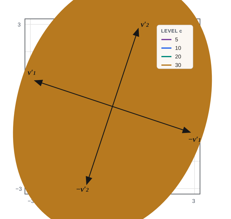
Nested elliptical level curves of a positive-definite quadratic form, together with its two orthogonal principal axes.
Four nested ellipses centered at the origin show the level sets \(q(x,y)=c\) for \(c=5,10,20,30\text{.}\) The first principal axis \(\mathbf{v}'_1=(-3,1)/\sqrt{10}\) runs from upper left to lower right, and the second principal axis \(\mathbf{v}'_2=(1,3)/\sqrt{10}\) runs from lower left to upper right. Each ellipse is shorter in the \(\mathbf{v}'_1\) direction, which has eigenvalue \(14\text{,}\) and longer in the \(\mathbf{v}'_2\) direction, which has eigenvalue \(4\text{.}\)
Figure 5.4.10. Level curves of \(q(x,y)=13x^2-6xy+5y^2\text{.}\) The principal-axis directions \(\mathbf{v}'_1\) and \(\mathbf{v}'_2\) are orthonormal eigenvectors of \(A\) with eigenvalues \(14\) and \(4\text{,}\) respectively.

Activity 5.4.11. Principal axes and level curves (U5-LO1, U5-LO4).

Consider the quadratic form
\begin{equation*} q(x,y) = x^2 + 4xy - 2y^2\text{.} \end{equation*}

(a)

Find the symmetric matrix \(A\) such that \(q = q_A\text{.}\)
Solution.
The matrix is
\begin{equation*} A = \begin{bmatrix} 1 \amp 2 \\ 2 \amp -2 \end{bmatrix}\text{.} \end{equation*}

(b)

Find the eigenvalues and corresponding eigenvectors of \(A\text{.}\)
Solution.
The characteristic polynomial is
\begin{align*} \det(A-\lambda I) \amp = \det \begin{bmatrix} 1-\lambda \amp 2\\ 2 \amp -2-\lambda \end{bmatrix}\\ \amp = (1-\lambda)(-2-\lambda)-4\\ \amp = \lambda^2+\lambda-6\\ \amp = (\lambda-2)(\lambda+3). \end{align*}
Thus the eigenvalues are \(2\) and \(-3\text{.}\) For eigenvalue \(\lambda_1 = 2\text{,}\) we solve \((A - \lambda_1 I)\mathbf{v}_1 = \mathbf{0}\text{:}\)
\begin{equation*} \begin{bmatrix} -1 \amp 2 \\ 2 \amp -4 \end{bmatrix}\begin{bmatrix} v_1 \\ v_2 \end{bmatrix} = \begin{bmatrix} 0 \\ 0 \end{bmatrix} \end{equation*}
That is, \(v_1 = 2v_2\text{.}\) Taking \(v_2 = 1\text{,}\) we get \(v_1 = 2\text{.}\) So
\begin{equation*} \mathbf{v}_1 = \begin{bmatrix} 2 \\ 1 \end{bmatrix} \end{equation*}
is an eigenvector for \(\lambda_1\text{.}\) For the eigenvalue \(\lambda_2 = -3\text{,}\) we solve \((A - \lambda_2 I)\mathbf{v}_2 = \mathbf{0}\text{:}\)
\begin{equation*} \begin{bmatrix} 4 \amp 2 \\ 2 \amp 1 \end{bmatrix}\begin{bmatrix} v_1 \\ v_2 \end{bmatrix} = \begin{bmatrix} 0 \\ 0 \end{bmatrix} \end{equation*}
That is, \(v_2 = -2v_1\text{.}\) Taking \(v_1 = 1\text{,}\) we get \(v_2 = -2\text{.}\) So an eigenvector for \(\lambda_2\) is \(\mathbf{v}_2 = \begin{bmatrix} 1 \\ -2 \end{bmatrix}\text{.}\)

(c)

Apply the previous theorem to express \(q(x_1, x_2)\) in terms of new coordinates \(y_1\) and \(y_2\) that eliminate the cross term, and classify the level curves \(q(x_1, x_2) = c\) for different values of \(c\text{.}\)
Solution.
We first normalize the eigenvectors to get:
\begin{align*} \mathbf{v}'_1 \amp = \frac{\mathbf{v}_1}{||\mathbf{v}_1||} = \frac{\begin{bmatrix} 2 \\ 1 \end{bmatrix}}{\sqrt{2^2 + 1^2}} = \frac{1}{\sqrt{5}}\begin{bmatrix} 2 \\ 1 \end{bmatrix}\\ \mathbf{v}'_2 \amp = \frac{\mathbf{v}_2}{||\mathbf{v}_2||} = \frac{\begin{bmatrix} 1 \\ -2 \end{bmatrix}}{\sqrt{1^2 + (-2)^2}} = \frac{1}{\sqrt{5}}\begin{bmatrix} 1 \\ -2 \end{bmatrix} \end{align*}
The orthogonal matrix \(Q\) with these unit eigenvectors as columns diagonalizes \(A\text{.}\) When we express a vector \(\mathbf{x} = Q\mathbf{y} = y_1\mathbf{v}'_1 + y_2\mathbf{v}'_2\text{,}\) the quadratic form becomes:
\begin{align*} q(\mathbf{x}) = \mathbf{x}^T A \mathbf{x} \amp = \mathbf{y}^T Q^T A Q \mathbf{y}\\ \amp = \mathbf{y}^T \begin{bmatrix} \lambda_1 \amp 0 \\ 0 \amp \lambda_2 \end{bmatrix} \mathbf{y}\\ \amp = \lambda_1 y_1^2 + \lambda_2 y_2^2\\ \amp = 2 y_1^2 - 3 y_2^2 \end{align*}
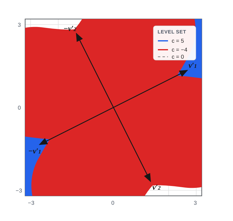
Hyperbolic level curves of an indefinite quadratic form, together with its principal axes and zero-level asymptotes.
The blue branches are the level set \(q(x,y)=5\) and open along \(\mathbf{v}'_1=(2,1)/\sqrt{5}\text{,}\) the eigenvector with positive eigenvalue \(2\text{.}\) The red branches are the level set \(q(x,y)=-4\) and open along \(\mathbf{v}'_2=(1,-2)/\sqrt{5}\text{,}\) the eigenvector with negative eigenvalue \(-3\text{.}\) Two dashed lines show the zero level set \(q(x,y)=0\text{;}\) these lines are asymptotes for the hyperbolas.
Figure 5.4.12. Level curves of \(q(x,y)=x^2+4xy-2y^2\text{.}\) In principal-axis coordinates, \(q=2y_1^2-3y_2^2\text{.}\)

Why is this true?.

By TheoremΒ 5.4.7, there is an orthogonal matrix \(Q\) such that
\begin{equation*} Q^TAQ=D=\operatorname{diag}(\lambda_1,\ldots,\lambda_n)\text{,} \end{equation*}
where \(\lambda_1,\ldots,\lambda_n\) are the eigenvalues of \(A\text{.}\) Set \(\mathbf{y}=Q^T\mathbf{x}\text{,}\) so \(\mathbf{x}=Q\mathbf{y}\text{.}\) Because \(Q\) is invertible, \(\mathbf{x}\neq\mathbf{0}\) if and only if \(\mathbf{y}\neq\mathbf{0}\text{.}\) The diagonalization theorem gives
\begin{equation*} \mathbf{x}^TA\mathbf{x} = \lambda_1y_1^2+\cdots+\lambda_ny_n^2. \end{equation*}
Suppose first that \(A\) is positive definite. Then every \(\lambda_i\) is strictly positive. If \(\mathbf{x}\neq\mathbf{0}\text{,}\) then \(\mathbf{y}\neq\mathbf{0}\text{,}\) so at least one coordinate \(y_i\) is nonzero. Therefore \(\lambda_1y_1^2+\cdots+\lambda_ny_n^2>0\text{,}\) and hence \(\mathbf{x}^TA\mathbf{x}>0\text{.}\)
Conversely, suppose \(\mathbf{x}^TA\mathbf{x}>0\) for every \(\mathbf{x}\neq\mathbf{0}\text{.}\) For each \(i\text{,}\) take \(\mathbf{y}=\mathbf{e}_i\) and \(\mathbf{x}=Q\mathbf{e}_i\text{.}\) Then \(\mathbf{x}\neq\mathbf{0}\) and
\begin{equation*} \mathbf{x}^TA\mathbf{x}=\lambda_i>0\text{.} \end{equation*}
Thus every eigenvalue of \(A\) is strictly positive, so \(A\) is positive definite.
The negative-definite case is analogous. If every \(\lambda_i\lt 0\text{,}\) then \(\lambda_1y_1^2+\cdots+\lambda_ny_n^2\lt 0\) for every \(\mathbf{y}\neq\mathbf{0}\text{,}\) so \(\mathbf{x}^TA\mathbf{x}\lt 0\) for every \(\mathbf{x}\neq\mathbf{0}\text{.}\) Conversely, if this quadratic form is strictly negative for every nonzero \(\mathbf{x}\text{,}\) taking \(\mathbf{x}=Q\mathbf{e}_i\) gives \(\lambda_i\lt 0\) for each \(i\text{.}\) Hence \(A\) is negative definite.
Note 5.4.14. Second-order optimization.

At a critical point, the linear part of the local approximation disappears. The next term is quadratic:
\begin{equation*} f(\mathbf{a}+\mathbf{h})\approx f(\mathbf{a})+\frac12\mathbf{h}^T H_f(\mathbf{a})\mathbf{h}. \end{equation*}
Thus the second derivative test is a linear algebra test applied to the Hessian matrix.

