MATH 345: Linear Algebra and Optimization

Section 3.6 Directional derivatives, critical points, and gradient descent

Subsection Directional derivatives

By DefinitionΒ 3.4.1, the first-order change in a scalar-valued function near \(\mathbf a\) is
\begin{equation*} f(\mathbf a+\mathbf h)-f(\mathbf a)\approx\nabla f(\mathbf a)^T\mathbf h. \end{equation*}
To study change along a unit direction \(\mathbf v\text{,}\) restrict the input to the line
\begin{equation*} \mathbf c(t)=\mathbf a+t\mathbf v. \end{equation*}
The resulting one-variable rate of change is the directional derivative.
The chain rule for one-parameter inputs in TheoremΒ 3.5.7 gives the gradient formula below.

Definition 3.6.1.

Let \(f\) be a scalar-valued function. Then if \(\mathbf{v}\) is a unit vector, the directional derivative of \(f\) in the direction of the vector \(\mathbf{v}\text{,}\) denoted \(D_{\mathbf{v}} f\text{,}\) is defined as
\begin{equation*} D_{\mathbf{v}} f(\mathbf{a}) = \lim_{h \to 0} \frac{f(\mathbf{a} + h \mathbf{v}) - f(\mathbf{a})}{h}\text{,} \end{equation*}
provided the limit exists.
The directional derivative represents the rate of change of the function \(f\) at the point \(\mathbf{a}\) in the direction of the unit vector \(\mathbf{v}\text{.}\) For a function \(f(x,y)\) of two variables, the directional derivative \(D_{\mathbf{v}} f(\mathbf{a})\) is the slope of the tangent line to the curve obtained by intersecting the surface \(z = f(x,y)\) with the plane containing both the line passing through \(\mathbf{a}\) with direction vector \(\mathbf{v}\text{,}\) and the \(z\) axis.

Remark 3.6.2.

Partial derivatives are a special case of directional derivatives, i.e., we have
\begin{equation*} \frac{\partial f}{\partial x_i} = D_{\mathbf{e}_i} f\text{.} \end{equation*}
Despite partial derivatives being a special case of directional derivatives, in most circumstances we can compute directional derivatives using partial derivatives, or equivalently, the gradient.

Why is this true?.

Define the path \(\mathbf{c}(t)=\mathbf{a}+t\mathbf{v}\) and the single-variable function \(g(t)=f(\mathbf{c}(t))=f(\mathbf{a}+t\mathbf{v})\text{.}\) Since \(\mathbf{c}(0)=\mathbf{a}\text{,}\) we have \(g(0)=f(\mathbf{a})\text{.}\) Therefore, the definition of the directional derivative gives
\begin{align*} D_{\mathbf{v}}f(\mathbf{a}) \amp= \lim_{h\to 0}\frac{f(\mathbf{a}+h\mathbf{v})-f(\mathbf{a})}{h}\\ \amp=\lim_{h\to 0}\frac{g(h)-g(0)}{h}\\ \amp=g'(0). \end{align*}
Write \(\mathbf{a}=(a_1,\ldots,a_n)\) and \(\mathbf{v}=(v_1,\ldots,v_n)\text{.}\) The \(i\)th coordinate of \(\mathbf{c}(t)\) is \(c_i(t)=a_i+tv_i\text{,}\) so \(c_i'(0)=v_i\text{.}\) Because \(g=f\circ\mathbf{c}\text{,}\) the chain rule (TheoremΒ 3.5.7) gives
\begin{align*} g'(0) \amp= \sum_{i=1}^n \frac{\partial f}{\partial x_i}(\mathbf{c}(0))c_i'(0)\\ \amp=\sum_{i=1}^n \frac{\partial f}{\partial x_i}(\mathbf{a})v_i\\ \amp=\nabla f(\mathbf{a})\cdot\mathbf{v}. \end{align*}
Combining the two calculations proves that \(D_{\mathbf{v}}f(\mathbf{a})=\nabla f(\mathbf{a})\cdot\mathbf{v}\text{.}\)
TheoremΒ 3.6.3 greatly simplifies the computations of directional derivatives.

Activity 3.6.4. Alignment with the gradient (U3-LO8, U1-LO1).

Suppose
\begin{equation*} \nabla f(\mathbf{a})=\begin{bmatrix}3\\4\end{bmatrix}. \end{equation*}
Compute \(D_{\mathbf{v}}f(\mathbf{a})\) for each unit vector below:
\begin{equation*} \mathbf{v}_1=\begin{bmatrix}1\\0\end{bmatrix}, \qquad \mathbf{v}_2=\begin{bmatrix}0\\1\end{bmatrix}, \qquad \mathbf{v}_3=\frac15\begin{bmatrix}3\\4\end{bmatrix}, \qquad \mathbf{v}_4=-\frac15\begin{bmatrix}3\\4\end{bmatrix}. \end{equation*}
Which listed direction gives the greatest increase? Which gives the greatest decrease?
Solution.
\begin{equation*} D_{\mathbf v_1}f(\mathbf a)=\begin{bmatrix}3\\4\end{bmatrix}\cdot\begin{bmatrix}1\\0\end{bmatrix}=3, \end{equation*}
and
\begin{equation*} D_{\mathbf v_2}f(\mathbf a)=\begin{bmatrix}3\\4\end{bmatrix}\cdot\begin{bmatrix}0\\1\end{bmatrix}=4. \end{equation*}
Also,
\begin{equation*} D_{\mathbf v_3}f(\mathbf a)=\begin{bmatrix}3\\4\end{bmatrix}\cdot\frac15\begin{bmatrix}3\\4\end{bmatrix}=5, \end{equation*}
while
\begin{equation*} D_{\mathbf v_4}f(\mathbf a)=-5. \end{equation*}
The greatest listed increase occurs in direction \(\mathbf v_3\text{,}\) which is aligned with the gradient. The greatest listed decrease occurs in direction \(\mathbf v_4\text{,}\) which points opposite the gradient.

Activity 3.6.5. Directional derivatives and unit directions (U3-LO8).

Let \(f(x,y) = x^2 y + y^2\text{.}\)
(a)
Compute the directional derivative \(D_{\mathbf{v}} f(1,2)\text{,}\) where \(\mathbf{v} = (1/\sqrt{2}, 1/\sqrt{2})\text{,}\) and \(f(x,y) = x^2y + y^2\text{.}\)
Solution.
We begin by computing the gradient of \(f\) at \((1,2)\text{.}\) We have
\begin{equation*} f_x(x,y) = 2xy \quad\text{and}\quad f_y(x,y) = x^2 + 2y\text{.} \end{equation*}
So \(\nabla f(x,y) = (2xy, x^2 + 2y)\text{,}\) and in particular
\begin{equation*} \nabla f(1,2) = \begin{bmatrix} 2(1)(2) \\ (1)^2 + 2 (2) \end{bmatrix} = \begin{bmatrix} 4 \\ 5 \end{bmatrix}\text{.} \end{equation*}
The given vector \(\mathbf{v}\) is already a unit vector because
\begin{equation*} \|\mathbf{v}\|=\sqrt{\left(\frac{1}{\sqrt{2}}\right)^2+\left(\frac{1}{\sqrt{2}}\right)^2}=1. \end{equation*}
Therefore, we may apply the directional-derivative formula directly:
\begin{equation*} D_{\mathbf{v}} f(1,2) = \nabla f(1,2) \cdot \mathbf{v} = \begin{bmatrix} 4 \\ 5 \end{bmatrix} \cdot \begin{bmatrix} 1/\sqrt{2} \\ 1/\sqrt{2} \end{bmatrix} = 9 / \sqrt{2}\text{.} \end{equation*}
(b)
Find the directional derivative of \(f\) at the point \((-1,3)\) in the direction of the vector \((-1,\sqrt{3})\text{.}\) That is, compute \(D_{\mathbf{v}} f(-1,3)\text{,}\) where \(\mathbf{v}\) is the unit vector in the direction of \((-1,\sqrt{3})\text{.}\)
Solution.
The vector
\begin{equation*} \begin{bmatrix} -1\\ \sqrt{3} \end{bmatrix} \end{equation*}
has norm
\begin{equation*} \sqrt{(-1)^2+(\sqrt{3})^2}=2\text{.} \end{equation*}
So the unit vector in this direction is
\begin{equation*} \mathbf{v} = \frac12 \begin{bmatrix} -1\\ \sqrt{3} \end{bmatrix} = \begin{bmatrix} -1/2\\ \sqrt{3}/2 \end{bmatrix}\text{.} \end{equation*}
For
\begin{equation*} f(x,y)=x^2y+y^2, \end{equation*}
we have
\begin{equation*} \nabla f(x,y)= \begin{bmatrix} 2xy\\ x^2+2y \end{bmatrix}. \end{equation*}
Thus
\begin{equation*} \nabla f(-1,3)= \begin{bmatrix} -6\\ 7 \end{bmatrix}. \end{equation*}
Therefore
\begin{equation*} D_{\mathbf{v}}f(-1,3) = \nabla f(-1,3)\cdot \mathbf{v} = \begin{bmatrix} -6\\ 7 \end{bmatrix} \cdot \begin{bmatrix} -1/2\\ \sqrt{3}/2 \end{bmatrix} = 3+\frac{7\sqrt{3}}{2} = \frac{6+7\sqrt{3}}{2}\text{.} \end{equation*}

Activity 3.6.6. A directional derivative between two points (U3-LO8).

Find the directional derivative of \(f\) at \((2,1)\) in the direction from \((2,1)\) to \((3,5)\text{.}\)
Solution.
The unit vector pointing in the direction from \((2,1)\) to \((3,5)\) is the unit vector pointing in the same direction as the vector \((3-2,5-1) = (1,4)\text{.}\) This vector has magnitude \(\sqrt{1^2 + 4^2} = \sqrt{17}\text{,}\) so the unit vector pointing in this direction is equal to
\begin{equation*} \mathbf{v} = \begin{bmatrix} 1/\sqrt{17}\\ 4/\sqrt{17} \end{bmatrix}\text{.} \end{equation*}
Now
\begin{equation*} \nabla f(x,y) = \begin{bmatrix} 3x^2 y\\ x^3 \end{bmatrix}\text{,} \end{equation*}
and in particular,
\begin{equation*} \nabla f(2,1) = \begin{bmatrix} 3(2)^2 (1)\\ (2)^3 \end{bmatrix} = \begin{bmatrix} 12\\ 8 \end{bmatrix}\text{.} \end{equation*}
So
\begin{equation*} D_{\mathbf{v}} f(2,1) = \nabla f(2,1) \cdot \mathbf{v} = \begin{bmatrix} 12\\ 8 \end{bmatrix} \cdot \begin{bmatrix} 1/\sqrt{17}\\ 4/\sqrt{17} \end{bmatrix} = \frac{12 + 32}{\sqrt{17}} = \frac{44}{\sqrt{17}}\text{.} \end{equation*}

Activity 3.6.7. Directional change toward a specified point (U3-LO8).

Let \(f(x,y)=x^2e^y\text{.}\) Find the directional derivative of \(f\) at \((2,0)\) in the direction pointing from \((2,0)\) to \((3,0)\text{.}\)
Solution.
A vector pointing from \((2,0)\) to \((3,0)\) is
\begin{equation*} \mathbf{d}= \begin{bmatrix} 3-2\\ 0-0 \end{bmatrix} = \begin{bmatrix} 1\\ 0 \end{bmatrix}. \end{equation*}
Its norm is
\begin{equation*} \|\mathbf{d}\|=\sqrt{1^2+0^2}=1. \end{equation*}
Thus this vector is already a unit vector. Therefore the required direction is
\begin{equation*} \mathbf{v}=\mathbf{d}= \begin{bmatrix} 1\\ 0 \end{bmatrix} =\mathbf{e}_1. \end{equation*}
Next,
\begin{equation*} \nabla f(x,y)= \begin{bmatrix} 2xe^y\\ x^2e^y \end{bmatrix}, \qquad \nabla f(2,0)= \begin{bmatrix} 4\\ 4 \end{bmatrix}. \end{equation*}
Thus
\begin{align*} D_{\mathbf{v}}f(2,0) \amp= \nabla f(2,0)\cdot\mathbf{v}\\ \amp=\begin{bmatrix}4\\4\end{bmatrix}\cdot\begin{bmatrix}1\\0\end{bmatrix}\\ \amp=4\cdot 1+4\cdot 0=4. \end{align*}

Why is this true?.

If \(\nabla f(\mathbf a)=\mathbf 0\text{,}\) then TheoremΒ 3.6.3 gives
\begin{equation*} D_{\mathbf v}f(\mathbf a)=0 \end{equation*}
for every unit vector \(\mathbf v\text{.}\)
Now suppose \(\nabla f(\mathbf a)\neq\mathbf 0\text{,}\) and let \(\theta\) be the angle between \(\nabla f(\mathbf a)\) and a unit vector \(\mathbf v\text{.}\) By TheoremΒ 3.6.3 and TheoremΒ 1.1.16,
\begin{equation*} D_{\mathbf v}f(\mathbf a)=\nabla f(\mathbf a)\cdot\mathbf v=\|\nabla f(\mathbf a)\|\cos\theta. \end{equation*}
The largest possible value of \(\cos\theta\) is \(1\text{,}\) attained when \(\mathbf v\) points in the direction of the gradient. The smallest possible value is \(-1\text{,}\) attained when \(\mathbf v\) points in the opposite direction. Therefore the maximum and minimum directional derivatives are
\begin{equation*} \|\nabla f(\mathbf a)\|\quad\text{and}\quad-\|\nabla f(\mathbf a)\|, \end{equation*}
attained at
\begin{equation*} \mathbf v=\frac{\nabla f(\mathbf a)}{\|\nabla f(\mathbf a)\|}\quad\text{and}\quad\mathbf v=-\frac{\nabla f(\mathbf a)}{\|\nabla f(\mathbf a)\|}, \end{equation*}
respectively.
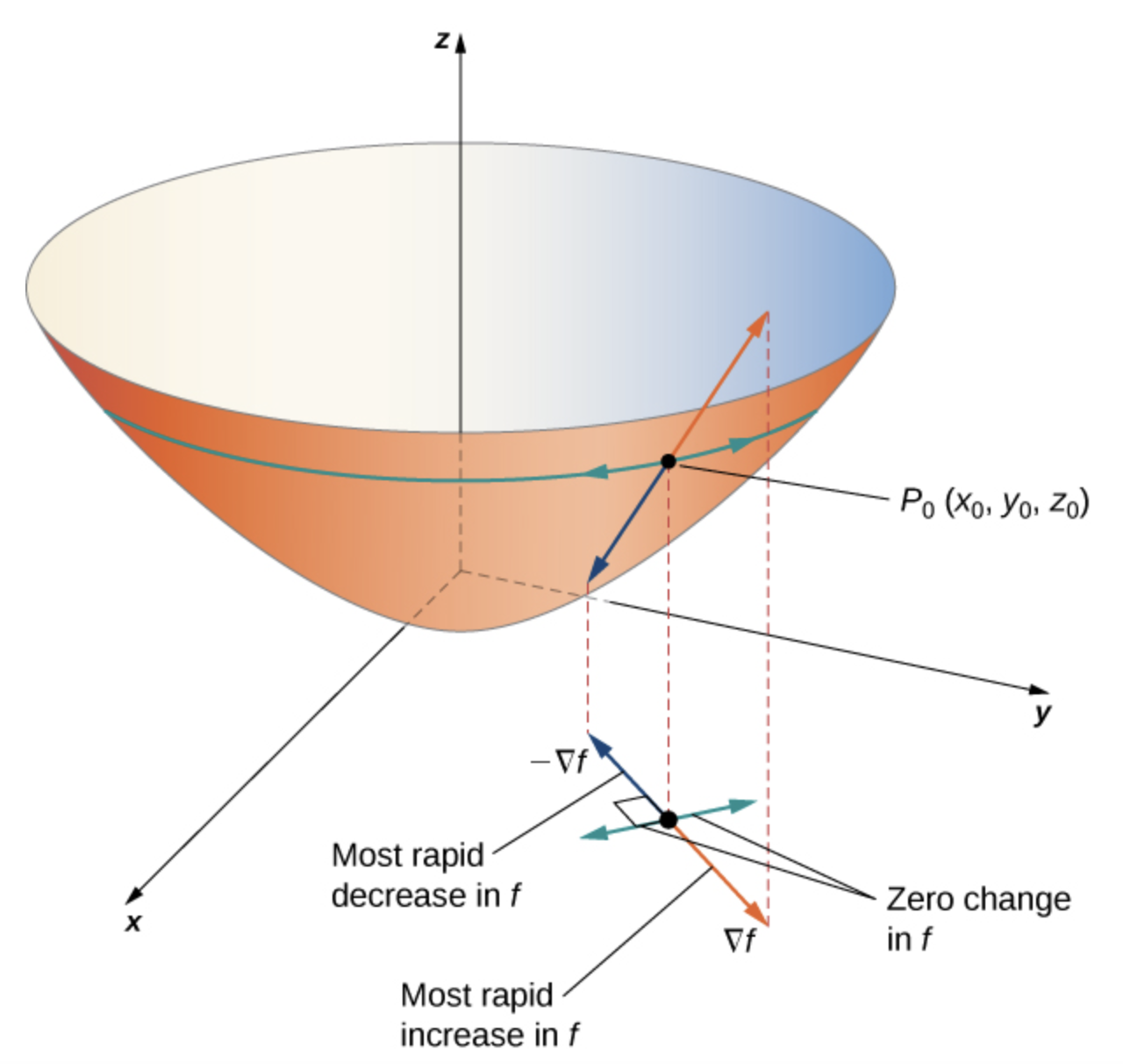
Gradient directions at a point on a surface.
A bowl-shaped surface is shown above the \(xy\)-plane with a point \(P_0(x_0,y_0,z_0)\) on the side of the surface. On the plane below, arrows based at the corresponding point show \(\nabla f\) for most rapid increase, \(-\nabla f\) for most rapid decrease, and perpendicular directions for zero change in \(f\text{.}\) Dashed vertical guide lines connect the point on the surface to its location in the domain.
Figure 3.6.9. The gradient indicates the maximum and minimum values of the directional derivative at a point. Figure 4.41 from Edwin β€œJed” Herman and Gilbert Strang, Calculus Volume 3, OpenStax, Β© 2018 Rice University, licensed under CC BY-NC-SA 4.0; source: OpenStax Figure 4.41.

Activity 3.6.10. Finding the direction of greatest increase (U3-LO8).

Find the direction for which the directional derivative of \(f(x,y) = 3x^2 - 4xy + 2y^2\) at \((-2,3)\) is a maximum. What is the maximum value of the directional derivative?
Solution.
First, we calculate that
\begin{equation*} \nabla f(x,y) = \begin{bmatrix} 6x - 4y\\ -4x + 4y \end{bmatrix}\text{.} \end{equation*}
So
\begin{equation*} \nabla f(-2,3) = \begin{bmatrix} 6(-2) - 4(3)\\ -4(-2) + 4(3) \end{bmatrix} = \begin{bmatrix} -24\\ 20 \end{bmatrix}\text{.} \end{equation*}
TheoremΒ 3.6.8 tells us that the directional derivative \(D_{\mathbf{v}} f\) is maximized when \(\mathbf{v}\) is the unit vector pointing in the direction of \((-24,20)\text{.}\) Since \((-24,20)\) has magnitude \(\sqrt{(-24)^2 + (20)^2} = \sqrt{976}\text{,}\) we see the direction which maximizes the directional derivative is
\begin{equation*} \mathbf{v} = \begin{bmatrix} -24/\sqrt{976}\\ 20/\sqrt{976} \end{bmatrix}\text{,} \end{equation*}
and the value of the directional derivative in this direction is equal to the magnitude of the gradient, which is
\begin{equation*} \sqrt{976}\text{.} \end{equation*}

Activity 3.6.11. A directional derivative in three variables (U3-LO8).

Calculate \(D_{\mathbf{u}}f(1, -2, 3)\) in the direction of \(\mathbf{v} = -\mathbf{i} + 2\mathbf{j} + 2\mathbf{k}\) for the function
\begin{equation*} f(x,y,z) = 5x^2 - 2xy + y^2 - 4yz + z^2 + 3xz. \end{equation*}
Solution.
We compute that
\begin{align*} \|\mathbf{v}\| \amp = \sqrt{(-1)^2 + (2)^2 + (2)^2} = \sqrt{9} = 3 \end{align*}
So the unit vector in the direction of \(\mathbf{v}\) is the vector
\begin{align*} \mathbf{u} \amp = \frac{\mathbf{v}}{\|\mathbf{v}\|} = -\frac{1}{3}\mathbf{i} + \frac{2}{3}\mathbf{j} + \frac{2}{3}\mathbf{k} \end{align*}
Using the formula for the directional derivative, we find that
\begin{align*} D_{\mathbf{u}}f(x,y,z) \amp = \nabla f(x,y,z) \cdot \mathbf{u}\\ \amp = \begin{bmatrix}10x - 2y\\ -2x + 2y - 4z\\ -4y + 2z + 3x\end{bmatrix} \cdot \mathbf{u}\\ \amp = - \frac{10x - 2y}{3} + 2 \frac{-2x + 2y - 4z}{3} + 2 \frac{-4y + 2z + 3x}{3}\text{.} \end{align*}
At the point \((1, -2, 3)\text{,}\) we evaluate that
\begin{equation*} D_{\mathbf{u}}f(1,-2,3) = (23)\left(-\frac{1}{3}\right) + (-18)\left(\frac{2}{3}\right) + (17)\left(\frac{2}{3}\right) = \frac{-25}{3} \end{equation*}
In SectionΒ 4.2, the same dot product will be interpreted as a signed projection coefficient of the gradient onto the chosen direction.

Subsection Optimization problems and critical points

Directional derivatives describe first-order change along a chosen direction. We now use them to identify candidates for local extrema and to motivate an iterative method for decreasing a function.
In this unit, we apply multivariate calculus to solve optimization problems.

Definition 3.6.12. Optimization problems.

Let \(f: \R^n \to \R\) be a scalar-valued function, and consider a set \(U \subseteq \R^n\text{.}\) Then we can consider two optimization problems, in which we call \(f\) the objective function of the problem, and \(U\) the feasible region of the optimization problem:
  • The minimization problem of \(f\) on \(U\) is the problem of finding \(\mathbf{x}^* \in U\) such that the value \(f(\mathbf{x}^*)\) is smallest among all elements of \(U\) (so the function is minimized on \(U\) by \(\mathbf{x}^*\)).
  • The maximization problem of \(f\) on \(U\) is the problem of finding \(\mathbf{x}^* \in U\) such that the value \(f(\mathbf{x}^*)\) is largest among all elements of \(U\) (so the function is maximized on \(U\) by \(\mathbf{x}^*\)).

Definition 3.6.13. Minima and maxima.

Suppose \(f\) is a scalar-valued function. A point \(\mathbf{a}\) in the domain of \(f\) is a
  • local minimum if there is a ball centered at \(\mathbf{a}\) such that \(f(\mathbf{a}) \leq f(\mathbf{x})\) whenever \(\mathbf{x}\) is in that ball and also in the domain of \(f\text{;}\) in other words, whenever \(\mathbf{x}\) is close enough to \(\mathbf{a}\) and lies in the domain of \(f\text{.}\) In this case, we say \(f(\mathbf{a})\) is a local minimum value for the function \(f\text{.}\)
  • local maximum if there is a ball centered at \(\mathbf{a}\) such that \(f(\mathbf{a}) \geq f(\mathbf{x})\) whenever \(\mathbf{x}\) is in that ball and also in the domain of \(f\text{;}\) in other words, whenever \(\mathbf{x}\) is close enough to \(\mathbf{a}\) and lies in the domain of \(f\text{.}\) In this case, we say \(f(\mathbf{a})\) is a local maximum value for the function \(f\text{.}\)
  • global minimum if \(f(\mathbf{a}) \leq f(\mathbf{x})\) for all \(\mathbf{x}\) in the domain of \(f\text{.}\) In this case, \(f(\mathbf{a})\) is the global minimum value, or absolute minimum value, of the function \(f\text{.}\)
  • global maximum if \(f(\mathbf{a}) \geq f(\mathbf{x})\) for all \(\mathbf{x}\) in the domain of \(f\text{.}\) In this case, \(f(\mathbf{a})\) is the global maximum value, or absolute maximum value, of the function \(f\text{.}\)
A local minimum or local maximum is also called a local extremum.

Remark 3.6.14.

The graph of the function \(-f\) is obtained by reflecting the graph of the function \(f\) in the output axis. This operation turns local and global maxima into local and global minima, and vice versa. So methods for finding minima for a general function often give methods for finding maxima, which makes the two problems often equivalent.

Definition 3.6.15. Critical points.

Suppose \(f\) is a scalar-valued function that is differentiable at a point \(\mathbf{a}\text{.}\) Then we say \(\mathbf{a}\) is a critical point if \(\nabla f(\mathbf{a}) = \mathbf{0}\text{.}\)
For a scalar-valued function of two variables, for example, \(f(x,y)\text{,}\) a critical point is a solution to the two equations \(f_x(x,y) = 0\) and \(f_y(x,y) = 0\text{.}\)
Just as the derivative of a scalar-valued function of a single variable helps identify local minima and maxima, partial derivatives provide information about possible local minima/maxima.

Why is this true?.

Let \(\mathbf v\) be a unit vector, and define
\begin{equation*} g(t)=f(\mathbf a+t\mathbf v). \end{equation*}
Because \(\mathbf a\) is an interior local extremum of \(f\text{,}\) the function \(g\) has a local extremum at \(t=0\text{.}\) Therefore
\begin{equation*} g'(0)=0. \end{equation*}
\begin{equation*} g'(0)=D_{\mathbf v}f(\mathbf a)=\nabla f(\mathbf a)\cdot\mathbf v. \end{equation*}
This holds for every unit vector \(\mathbf v\text{.}\) If \(\nabla f(\mathbf a)\neq\mathbf 0\text{,}\) choose
\begin{equation*} \mathbf v=\frac{\nabla f(\mathbf a)}{\|\nabla f(\mathbf a)\|}. \end{equation*}
Then
\begin{equation*} \nabla f(\mathbf a)\cdot\mathbf v=\|\nabla f(\mathbf a)\|>0, \end{equation*}
a contradiction. Hence \(\nabla f(\mathbf a)=\mathbf0\text{.}\)

Activity 3.6.17. Critical points of a quadratic function (U3-LO9).

Find the critical points of the function
\begin{equation*} f(x,y) = x^2 + y^2 - 2x + 4y\text{.} \end{equation*}
Solution.
To find the critical points, we calculate the partial derivatives and set them equal to zero. We find that
\begin{equation*} f_x(x,y) = 2x - 2 \quad\text{and}\quad f_y(x,y) = 2y + 4\text{.} \end{equation*}
The critical points are the pairs \((x,y)\) that simultaneously solve the equations \(2x - 2 = 0\) and \(2y + 4 = 0\text{.}\) So the only critical point is \((1, -2)\text{.}\)

Activity 3.6.18. Critical points of a difference of squares (U3-LO9).

Find the critical points of \(f(x,y) = x^2 - y^2\text{.}\)
Solution.
We compute that \(f_x(x,y) = 2x\) and \(f_y(x,y) = -2y\text{.}\) The only \((x,y)\) such that \(f_x(x,y) = 2x = 0\) and \(f_y(x,y) = -2y = 0\) is \((0,0)\text{.}\) This is the only critical point.

Warning 3.6.19. Critical points are candidates.

The equation \(\nabla f=0\) finds candidates for local extrema. It does not by itself find boundary extrema, constrained extrema, or absolute extrema. Always combine critical-point information with the domain and boundary conditions.

Subsection Gradient descent

Activity 3.6.20. Critical-point equations in three variables (U3-LO9).

Find the system of equations satisfied by the critical points of the function
\begin{equation*} f(x,y,z) = x^2e^{yz} + y\sin(xz) + z\cos(xy)\text{.} \end{equation*}
Solution.
We calculate that
\begin{equation*} f_x(x,y,z)=2xe^{yz}+yz\cos(xz)-yz\sin(xy)\text{,} \end{equation*}
that
\begin{equation*} f_y(x,y,z)=x^2ze^{yz}+\sin(xz)-xz\sin(xy) \end{equation*}
and that
\begin{equation*} f_z(x,y,z)=x^2ye^{yz}+xy\cos(xz)+\cos(xy)\text{.} \end{equation*}
So the critical points of \(f\) are the solutions to the system of equations
\begin{equation*} \begin{cases} 2xe^{yz}+yz\cos(xz)-yz\sin(xy)=0,\\ x^2ze^{yz}+\sin(xz)-xz\sin(xy)=0,\\ x^2ye^{yz}+xy\cos(xz)+\cos(xy)=0. \end{cases} \end{equation*}
Using the calculus we have developed, it is usually straightforward to write the equations that critical points must satisfy. ActivityΒ 3.6.20 also shows the problem: those equations may be nonlinear and difficult or impossible to solve exactly. This is different from the linear systems in Unit 2, where Gaussian elimination gave a systematic exact method.
When the critical-point equations cannot be solved directly, one often uses a numerical method. By TheoremΒ 3.6.8, the negative gradient gives the direction of steepest local decrease.
At a current point \(\mathbf x_k\text{,}\) choose
\begin{equation*} \mathbf h=-\alpha\nabla f(\mathbf x_k),\qquad \alpha>0. \end{equation*}
\begin{align*} f(\mathbf x_k+\mathbf h)-f(\mathbf x_k) \amp\approx \nabla f(\mathbf x_k)^T\mathbf h\\ \amp=-\alpha\|\nabla f(\mathbf x_k)\|^2. \end{align*}
Unless the gradient is zero, the local model predicts a decrease. This is a local prediction, not a convergence theorem. It motivates the gradient-descent update
\begin{equation*} \mathbf x_{k+1}=\mathbf x_k-\alpha\nabla f(\mathbf x_k). \end{equation*}
The gradient-descent algorithm repeats this local step.
  1. Start at an initial point \(\mathbf{x}_0\text{.}\)
  2. Compute the gradient \(\nabla f(\mathbf{x}_0)\text{.}\)
  3. Move in the direction of the negative gradient: set \(\mathbf{x}_1 = \mathbf{x}_0 - \alpha_0 \nabla f(\mathbf{x}_0)\text{,}\) where \(\alpha_0 > 0\) is a step size (or learning rate) parameter.
  4. Repeat steps 2-3 with step sizes \(\alpha_1, \alpha_2, \dots\) to successively define points \(\mathbf{x}_2 = \mathbf{x}_1 - \alpha_1 \nabla f(\mathbf{x}_1)\text{,}\) \(\mathbf{x}_3 = \mathbf{x}_2 - \alpha_2 \nabla f(\mathbf{x}_2)\text{,}\) and so on, with the hope that these points converge to a local minimum.
In data and modeling problems, an objective function being minimized is often called a loss.
Intuitively, gradient descent works because each successive value \(\mathbf{x}_k\) is obtained by shifting the previous value \(\mathbf{x}_{k-1}\) in the direction in which the function \(f\) decreases the fastest. Gradient descent may converge to a local minimum under additional assumptions on the function and the learning rates. The examples below illustrate possible behavior; they do not prove convergence.

Activity 3.6.21. Reading one gradient descent update (U3-LO8, U3-LO9).

Assume grad_f(x) computes \(\nabla f(\mathbf{x})\text{.}\) Consider the line of code
x = x - alpha * grad_f(x)
  1. What mathematical update rule does this line represent?
  2. Which quantity is the learning rate?
  3. Why must grad_f(x) have the same shape as x?
  4. What would change if the minus sign were a plus sign?
Solution.
The line represents the update
\begin{equation*} \mathbf{x}_{k+1}=\mathbf{x}_k-\alpha\nabla f(\mathbf{x}_k). \end{equation*}
The learning rate is alpha. The vector grad_f(x) must have the same shape as x, because the update subtracts one vector from another. If the minus sign were a plus sign, the update would move in the direction of steepest increase rather than steepest decrease.

Activity 3.6.22. Three gradient-descent steps (U3-LO9).

Find an approximate minimum of the function \(f : \R^2 \to \R\) defined by
\begin{equation*} f(x, y) = x^2 - 3xy + 3y^2 + 5y + 2x \end{equation*}
using gradient descent. Use the starting point \(\mathbf{x}_0 = (0,0)\text{,}\) a constant step size of \(0.1\text{,}\) and stop after computing \(\mathbf{x}_3\text{.}\) You may use a calculator to perform these computations.
Solution.
First, we calculate the gradient:
\begin{equation*} \nabla f(x, y) = \begin{bmatrix} 2x - 3y + 2 \\ -3x + 6y + 5 \end{bmatrix} \end{equation*}
Starting at \(\mathbf{x}_0 = (0,0)\text{,}\) we successively compute that
\begin{equation*} \nabla f(0,0) = \begin{bmatrix} 2 \\ 5 \end{bmatrix}\text{,} \end{equation*}
so
\begin{equation*} \mathbf{x}_1 = \begin{bmatrix}0\\0\end{bmatrix} - 0.1\begin{bmatrix} 2 \\ 5 \end{bmatrix} = \begin{bmatrix} -0.2 \\ -0.5 \end{bmatrix}\text{.} \end{equation*}
We then compute that
\begin{equation*} \nabla f(-0.2,-0.5) = \begin{bmatrix} -0.4-(-1.5)+2 \\ -3(-0.2)+6(-0.5)+5 \end{bmatrix} = \begin{bmatrix} 3.1 \\ 2.6 \end{bmatrix}\text{,} \end{equation*}
so
\begin{equation*} \mathbf{x}_2 = \begin{bmatrix} -0.2 \\ -0.5 \end{bmatrix} - 0.1\begin{bmatrix} 3.1 \\ 2.6 \end{bmatrix} = \begin{bmatrix} -0.51 \\ -0.76 \end{bmatrix}\text{.} \end{equation*}
Finally, we compute that
\begin{equation*} \nabla f(-0.51,-0.76) = \begin{bmatrix} 2(-0.51) - 3(-0.76) + 2 \\ -3(-0.51) + 6(-0.76) + 5 \end{bmatrix} = \begin{bmatrix} 3.26 \\ 1.97 \end{bmatrix}\text{,} \end{equation*}
so
\begin{equation*} \mathbf{x}_3 = \begin{bmatrix} -0.51 \\ -0.76 \end{bmatrix} - 0.1\begin{bmatrix} 3.26 \\ 1.97 \end{bmatrix} = \begin{bmatrix} -0.836 \\ -0.957 \end{bmatrix}\text{.} \end{equation*}
In ActivityΒ 5.5.19, we compute exactly that the unique critical point is
\begin{equation*} \left(-9,-\frac{16}{3}\right) \end{equation*}
and classify it after developing second-order tools. Thus \(\mathbf x_3\) is not yet a good approximation. If we continue the iteration, the points \(\mathbf x_k\) for, say, \(k\geq1000\) are very close to that critical point.

Remark 3.6.23.

The iteration is cumbersome by hand but easy to repeat on a computer when the gradient is available.
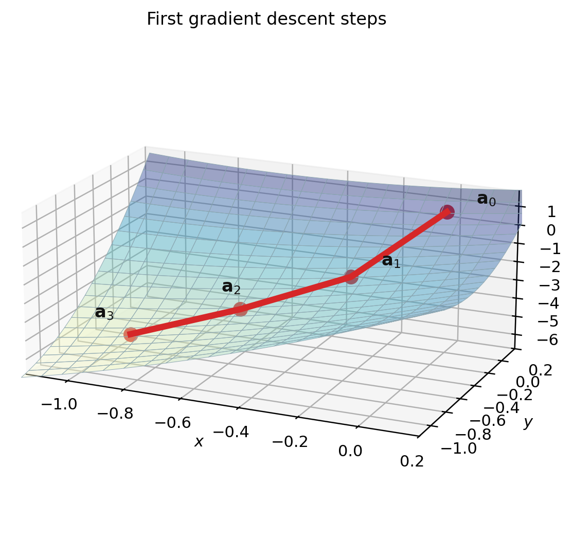
Surface plot showing the first gradient descent steps from the origin.
The figure shows a side view of the surface \(z=f(x,y)\) for \(f(x,y)=x^2-3xy+3y^2+5y+2x\) over a small region near the origin. Four red points labeled \(\mathbf{x}_0\text{,}\) \(\mathbf{x}_1\text{,}\) \(\mathbf{x}_2\text{,}\) and \(\mathbf{x}_3\) are connected by red line segments on the surface, showing the first three gradient descent steps from \((0,0)\text{.}\)
Figure 3.6.24. Initial steps of gradient descent for \(f(x,y)=x^2-3xy+3y^2+5y+2x\) with starting point \(\mathbf{x}_0 = (0, 0)\text{.}\) For \(k=1,2,3\text{,}\) the point \(\mathbf{x}_k\) is determined by the rule \(\mathbf{x}_k = \mathbf{x}_{k-1} - (0.1) \nabla f(\mathbf{x}_{k-1})\text{.}\) Adapted from Stanford’s MATH 51 textbook.